Image Transforms Transforming images to images Classification of

Image Transforms Transforming images to images

Classification of Image Transforms • Point transforms – modify individual pixels – modify pixels’ locations • Local transforms – output derived from neighbourhood • Global transforms – whole image contributes to each output value

Point Transforms • Manipulating individual pixel values – Brightness adjustment – Contrast adjustment • Histogram manipulation – equalisation • Image magnification

Monadic, Point-by-point Operators • Monadic point-to-point operator

Brightness Adjustment Add a constant to all values g’ = g + k (k = 50)

Contrast Adjustment Scale all values by a constant g’ = g*k (k = 1. 5)

Contrast Enhancement • • • Add Subtract Multiply Divide Maximum Minimum

A sub-image (x-1, y-1) (x+1, y-1) (x-1, y) (x+1, y) (x-1, y+1) (x+1, y+1)

Intensity Shift C(x, y) <= 0 a(x, y)+k < 0 a(x, y) +k 0<=a(x, y) +k <=W W W<a(x, y) +k Where k is a user defined variable

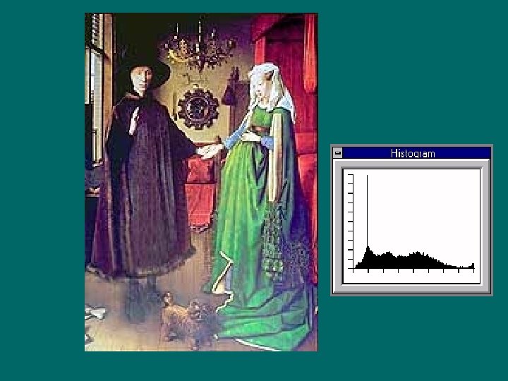
Image Histogram • Measure frequency of occurrence of each grey/colour value

Histogram Manipulation • Modify distribution of grey values to achieve some effect

Histogram Equalization • An important operator for image enhancement is given by the transformation: • C(x, y)<= W x H (a(x, y)) mxn

Equalisation/Adaptive Equalisation • Specifically to make histogram uniform

Retrieval based on colour • Retrieval by colour similarity requires that models of colour stimuli are used, such that distances in the colour space correspond to human perceptual distances between colours. • Colour patterns must be represented in such a way that salient chromatic properties are captured.

Colour Histogram • Application example - colour histogram retrieval: This method is to retrieve images from the database that have perceptually similar colour to the input image or input description from the user. • The basic idea is to quantize each of the RGB values into m intervals resulting in a total number of m 3 colour combinations (or bins) • A colour histogram H(I) is then constructed. This colour histogram is a vector {h 1, h 2, …, hm 3} where element hx represents the number of pixels in image I falling within bin x.

Colour Histogram • • • The colour histogram becomes the index of this image To retrieve image from the database, the user supplies either a sample image or a specification for the system to construct a colour histogram H(Q). A distance metric is used to measure the similarity between H(Q) and H(I). Where I represents each of the images in the database. And example distance metric is shown as follows: x=m 3 D(Q, I ) = |qx-ix| x=1 Where qx and ix are the numbers of pixels in the image Q and I, respectively, falling within bin x.

Colour Histogram • • may fail in recognizing images with perceptually similar colours but no common colours. This may be due to a shift in colour values, noise or change in illumination. – measure the similarity Not enough for complicated images where spatial position is more important information. – May consider dividing each image into multiple regions and compare the colour histograms of the same regions in the images. • May combine with other methods such as shape and/or texture based retrieval to improve the accuracy of the retrieval.

Threshold • This is an important function, which converts a grey scale image to a binary format. Unfortunately, it is often difficult, or even impossible to find satisfactory values for the user defined integer threshold value

Threshold • C(x, y) <= W a(x, y)>=threshold 0 otherwise for (int y=0; y<height; y++) for(int x=0; x<width; x++) if (input. getxy(x, y) < threshold) output. setxy(x, y, BLACK); else output. setxy(x, y, WHITE);

Thresholding • Transform grey/colour image to binary if f(x, y) > T output = 1 else 0 • How to find T?

Threshold Value • Manual – User defines a threshold • P-Tile • Mode • Other automatic methods

Image Magnification • Reducing – new value is weighted sum of nearest neighbours – new value equals nearest neighbour • Enlarging – new value is weighted sum of nearest neighbours – add noise to obscure pixelation

Local Transforms • Convolution • Applications – smoothing – sharpening – matching

Local Operators • The concept behind local operators is that the intensities of several pixels are combined together in order to calculate the intensity of just one pixel. Amongst the simplest of the local operators are those which use a set of nine pixels arranged in a 3 x 3 square region. It computes the value for one pixel on the basis of the intensities within a region containing 3 x 3 pixels. Other local operators employ larger windows.

Local Operators

Convolution Definition Place template on image Multiply overlapping values in image and template Sum products and normalise (Templates usually small)

Example Image …. … 3 … 4 … 4 …. . 5 5 6 6 5. . 7 8 9 9 8. Template. 4 5 6 5 5. . . 4… 4… 4… 3… 4…. . 1 1 2 1 Result 1 1 1 … … … … Divide by template sum . . 6 6 6. . 6 7 7. . 6 6 6. . . …. …. …. . . .

Separable Templates • Convolve with n x n template – n 2 multiplications and additions • Convolve with two n x 1 templates – 2 n multiplications and additions

Example • Laplacian template 0 – 1 0 -1 4 – 1 0 • Separated kernels -1 2 -1

Applications • Usefulness of convolution is the effects generated by changing templates – Smoothing • Noise reduction – Sharpening • Edge enhancement

Smoothing • Aim is to reduce noise • What is “noise”? • How is it reduced – Addition – Adaptively – Weighted

Noise Definition • Noise is deviation of a value from its expected value – Random changes • x x+n – Salt and pepper • x {max, min}

Noise Reduction • By smoothing (x + n) = (x) + (n) = (x) – Since noise is random and zero mean • Smooth locally or temporally • Local smoothing – Removes detail – Introduces ringing

Adaptive Smoothing • Compute smoothed value, s • Output = s if |s – x| > T x otherwise

Median Smoothing Median is one value in an ordered set: 1 2 3 4 5 6 7 median = 4. 5

Original Smoothed Median Smoothing

Sharpening • What is it? – Enhancing discontinuities – Edge detection • Why do it? – Perceptually important – Computationally important

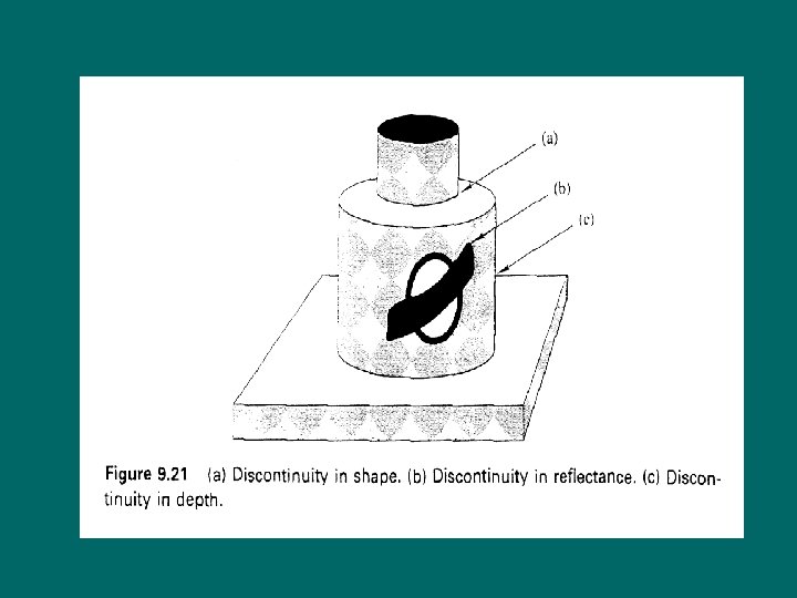
Edge Definition An edge is a significant local change in image intensity.

Algorithms for Edge Detection • Algorithms for detecting edges - edge detectors – differentiation based • estimated the derivatives of the image intensity function, the idea being that large image derivatives reflect abrupt intensity changes. – Model based • determine whether the intensities in a small area conform to some model for the edges that we have assumed.

First Derivative, Gradient Edge Detection • If an edge is a discontinuity • Can detect it by differencing

Roberts Cross Edge Detector -1 0 0 -1 0 1 1 • Simplest edge detector • Inaccurate localisation 0

Prewitt/Sobel Edge Detector -1 -1 -1 0 0 0 1 1 1 -1 0 1 1 1

Edge Detection • Combine horizontal and vertical edge estimates

Example Results

Example Results

Global Transforms • Computing a new value for a pixel using the whole image as input • Cosine and Sine transforms • Fourier transform – Frequency domain processing • Hough transform • Karhunen-Loeve transform • Wavelet transform

Geometric Transformations • Definitions – Affine and non-affine transforms • Applications – Manipulating image shapes

Affine Transforms Scale, Shear, Rotate, Translate Length and areas preserved. x’ = a b c x y’ d e f y 1 g h i 1 Change values of transform matrix elements according to desired effect. [ ][ ] a, e scaling b, d shearing a, b, d, e rotation c, f translation

Affine Transform Examples

Warping Example Ansell Adams’ Aspens

Image Resampling • Moving source to destination pixels • x’ and y’ could be non-integer • Round result – can create holes in image • Manipulate in reverse – where did warped pixel come from – source is non-integer • interpolate nearest neighbours

Summary • Point transforms – scaling, histogram manipulation, thresholding • Local transforms – edge detection, smoothing • Global transforms – Fourier, Hough, Principal Component, Wavelet • Geometrical transforms