Convolutional Neural Networks CSE 4310 Computer Vision Vassilis

Convolutional Neural Networks CSE 4310 – Computer Vision Vassilis Athitsos Computer Science and Engineering Department University of Texas at Arlington 1

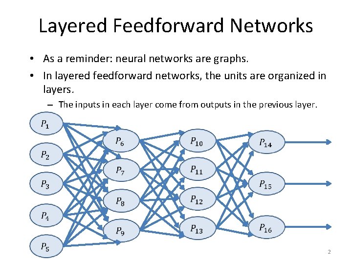
Layered Feedforward Networks • As a reminder: neural networks are graphs. • In layered feedforward networks, the units are organized in layers. – The inputs in each layer come from outputs in the previous layer. 2

Design Choices • Some important design choices in a neural network: – Number of layers. • Too many: slow to train, risk of overfitting. 3

Design Choices • Some important design choices in a neural network: – Number of layers. • Too many: slow to train, risk of overfitting. • Here we need a necessary parenthesis: what is overfitting? 4

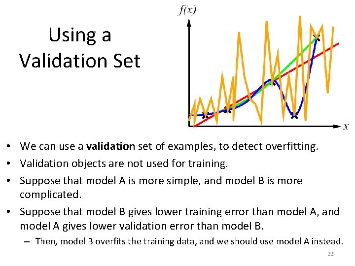
Overfitting • Some important design choices in a neural network: – Number of layers. • Too many: slow to train, risk of overfitting. • What is overfitting? – Overfitting is the commonly occurring phenomenon in machine learning where, after training, we get a model that works much better on the training data than on test data. • Why does overfitting happen? – If our model has too many degrees of freedom, fitting the training data very well does not automatically imply that it will fit test data very well. 5

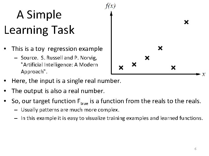
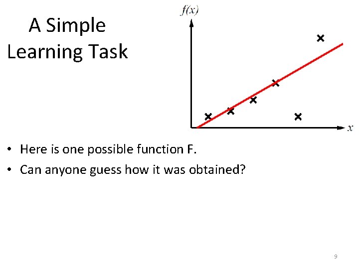
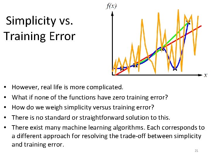
A Simple Learning Task • This is a toy regression example. . – Source. S. Russell and P. Norvig, "Artificial Intelligence: A Modern Approach". • Here, the input is a single real number. • The output is also a real number. • So, our target function Ftrue is a function from the reals to the reals. – Usually patterns are much more complex. – In this example it is easy to visualize training examples and learned functions. 6

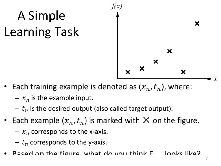
A Simple Learning Task • 7

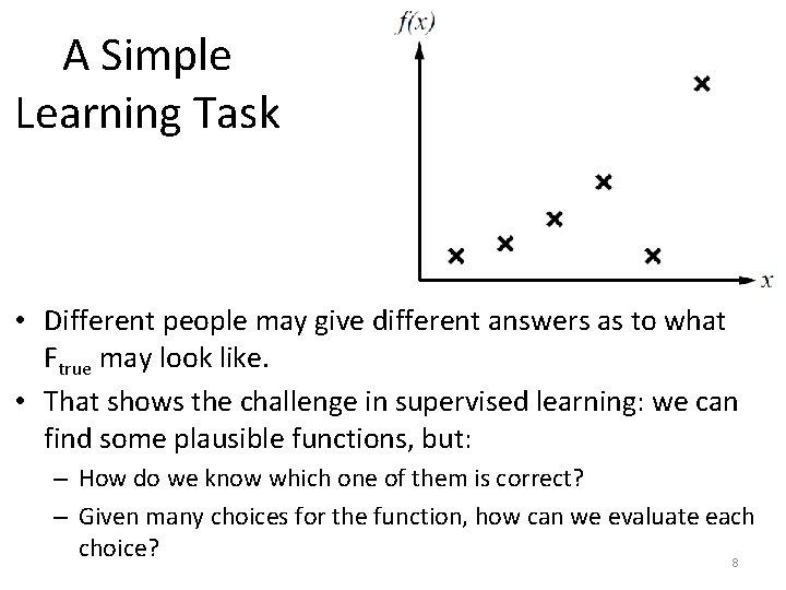
A Simple Learning Task • Different people may give different answers as to what Ftrue may look like. • That shows the challenge in supervised learning: we can find some plausible functions, but: – How do we know which one of them is correct? – Given many choices for the function, how can we evaluate each choice? 8

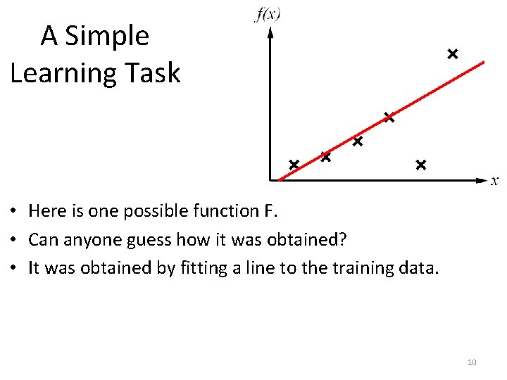
A Simple Learning Task • Here is one possible function F. • Can anyone guess how it was obtained? 9

A Simple Learning Task • Here is one possible function F. • Can anyone guess how it was obtained? • It was obtained by fitting a line to the training data. 10

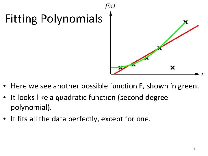
Fitting Polynomials • Here we see another possible function F, shown in green. • It looks like a quadratic function (second degree polynomial). • It fits all the data perfectly, except for one. 11

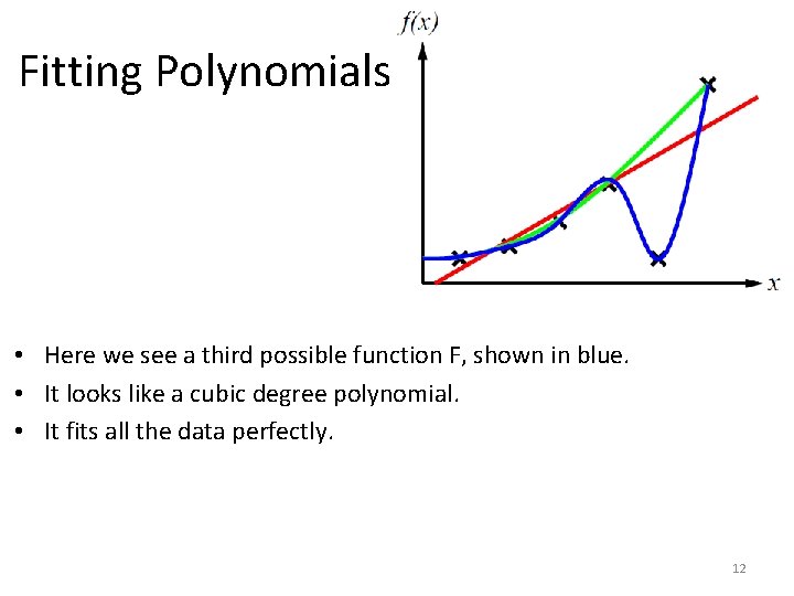
Fitting Polynomials • Here we see a third possible function F, shown in blue. • It looks like a cubic degree polynomial. • It fits all the data perfectly. 12

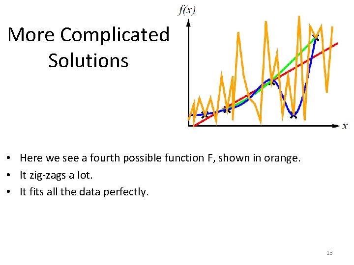
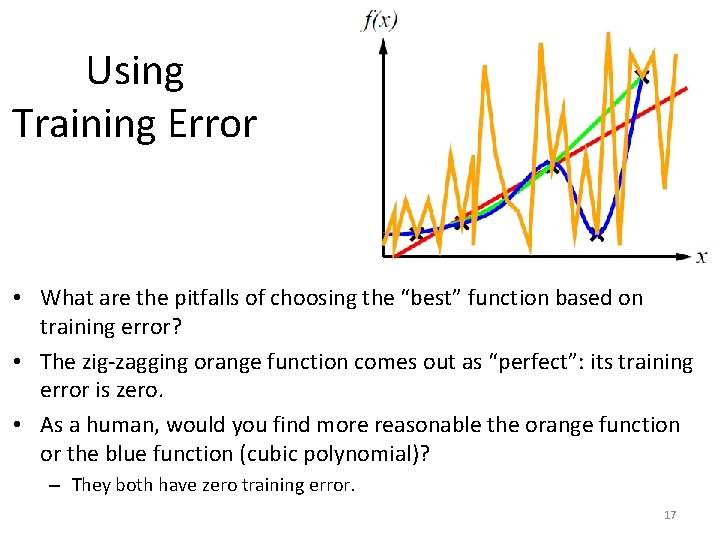
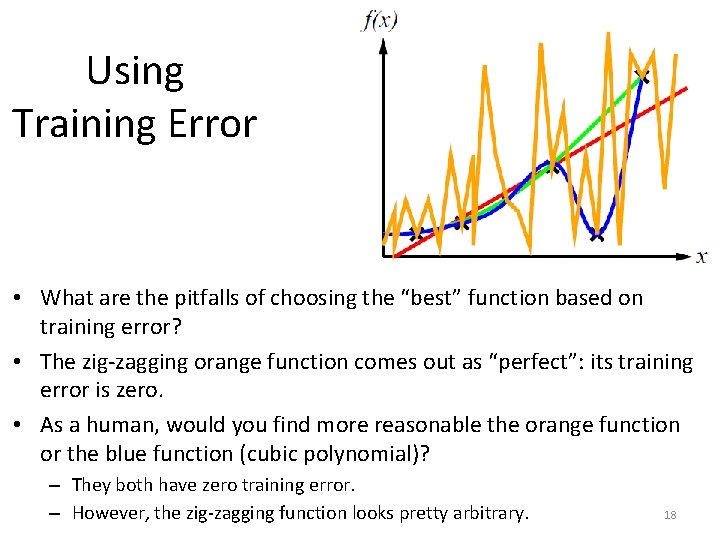
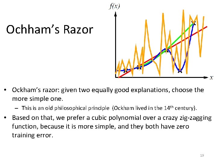
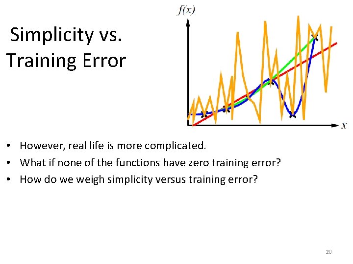
More Complicated Solutions • Here we see a fourth possible function F, shown in orange. • It zig-zags a lot. • It fits all the data perfectly. 13

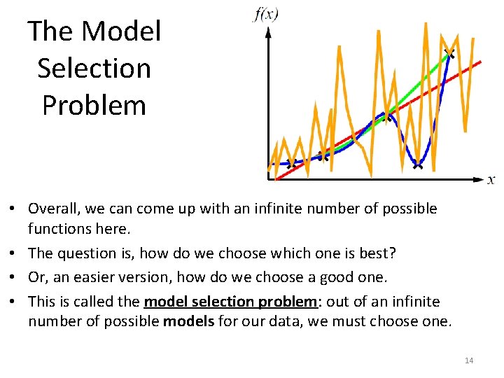
The Model Selection Problem • Overall, we can come up with an infinite number of possible functions here. • The question is, how do we choose which one is best? • Or, an easier version, how do we choose a good one. • This is called the model selection problem: out of an infinite number of possible models for our data, we must choose one. 14

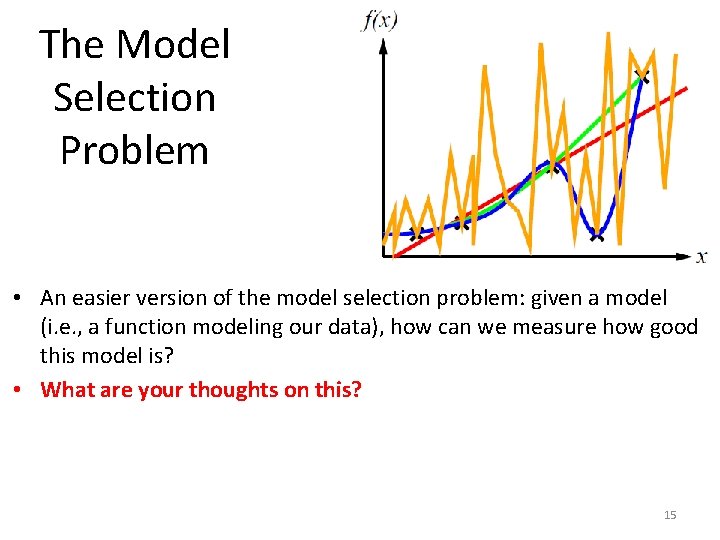
The Model Selection Problem • An easier version of the model selection problem: given a model (i. e. , a function modeling our data), how can we measure how good this model is? • What are your thoughts on this? 15

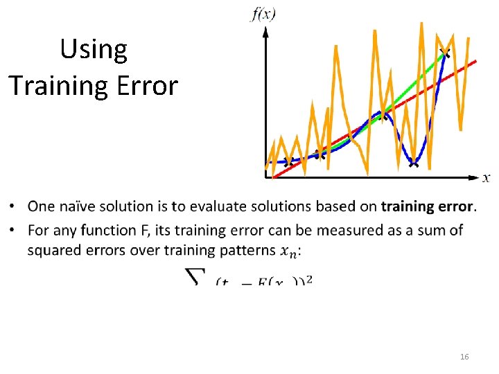
Using Training Error • 16

Using Training Error • What are the pitfalls of choosing the “best” function based on training error? • The zig-zagging orange function comes out as “perfect”: its training error is zero. • As a human, would you find more reasonable the orange function or the blue function (cubic polynomial)? – They both have zero training error. 17

Using Training Error • What are the pitfalls of choosing the “best” function based on training error? • The zig-zagging orange function comes out as “perfect”: its training error is zero. • As a human, would you find more reasonable the orange function or the blue function (cubic polynomial)? – They both have zero training error. – However, the zig-zagging function looks pretty arbitrary. 18

Ochham’s Razor • Ockham’s razor: given two equally good explanations, choose the more simple one. – This is an old philosophical principle (Ockham lived in the 14 th century). • Based on that, we prefer a cubic polynomial over a crazy zig-zagging function, because it is more simple, and they both have zero training error. 19

Simplicity vs. Training Error • However, real life is more complicated. • What if none of the functions have zero training error? • How do we weigh simplicity versus training error? 20

Simplicity vs. Training Error • • • However, real life is more complicated. What if none of the functions have zero training error? How do we weigh simplicity versus training error? There is no standard or straightforward solution to this. There exist many machine learning algorithms. Each corresponds to a different approach for resolving the trade-off between simplicity and training error. 21

Using a Validation Set • We can use a validation set of examples, to detect overfitting. • Validation objects are not used for training. • Suppose that model A is more simple, and model B is more complicated. • Suppose that model B gives lower training error than model A, and model A gives lower validation error than model B. – Then, model B overfits the training data, and we should use model A instead. 22

Design Choices • Some important design choices in a neural network: – Number of layers. • Too many: slow to train, risk of overfitting. 23

Design Choices • Some important design choices in a neural network: – Number of layers. • Too many: slow to train, risk of overfitting. • Too few: may be too simple to learn an accurate model. 24

Design Choices • Some important design choices in a neural network: – Number of layers. • Too many: slow to train, risk of overfitting. • Too few: may be too simple to learn an accurate model. – Number of units per layer. • • We have a separate choice for each layer. Too many: slow to train, dangers of overfitting. Too few: may be too simple to learn an accurate model. We have no choice for input layer (number of units = number of dimensions of input vectors) and output layer (number of units = number of classes). – Connectivity: what outputs are connected to what inputs? 25

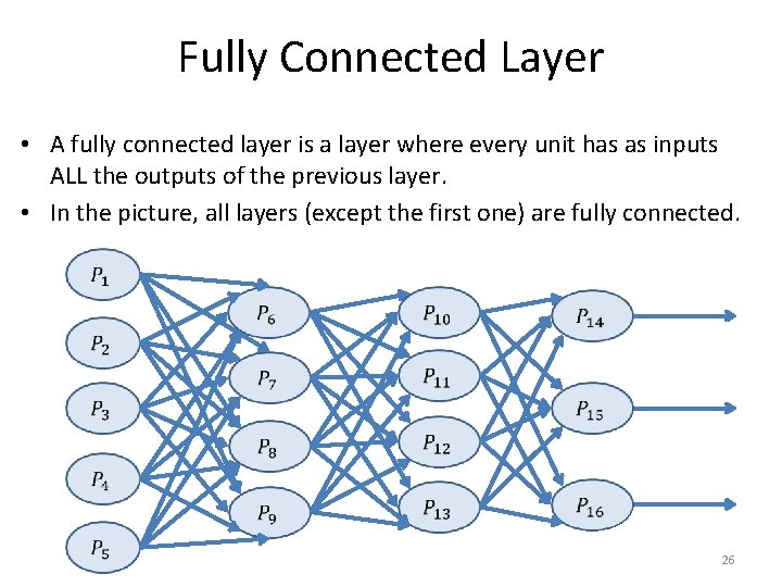
Fully Connected Layer • A fully connected layer is a layer where every unit has as inputs ALL the outputs of the previous layer. • In the picture, all layers (except the first one) are fully connected. 26

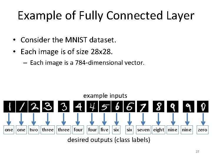
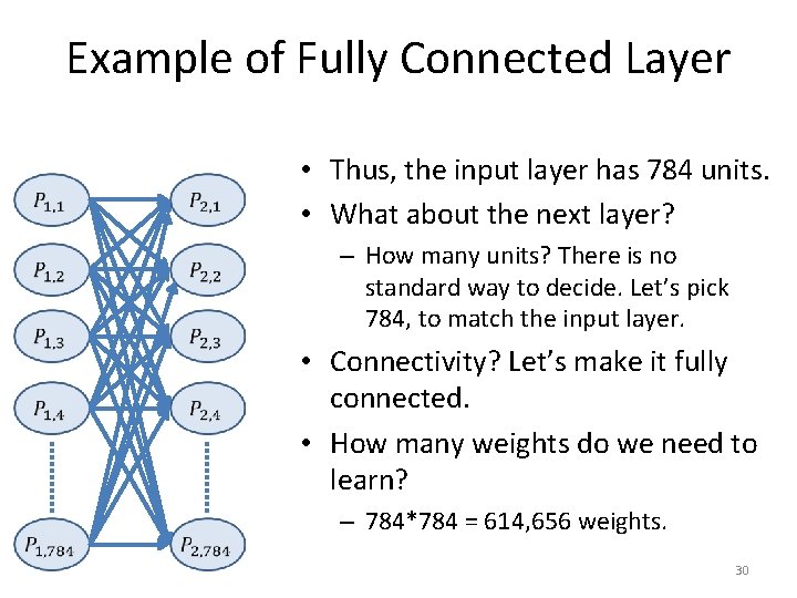
Example of Fully Connected Layer • Consider the MNIST dataset. • Each image is of size 28 x 28. – Each image is a 784 -dimensional vector. example inputs one two three four five six seven eight nine zero desired outputs (class labels) 27

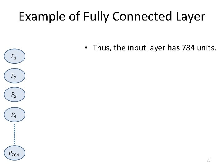
Example of Fully Connected Layer • Thus, the input layer has 784 units. 28

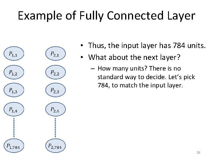
Example of Fully Connected Layer • Thus, the input layer has 784 units. • What about the next layer? – How many units? There is no standard way to decide. Let’s pick 784, to match the input layer. 29

Example of Fully Connected Layer • Thus, the input layer has 784 units. • What about the next layer? – How many units? There is no standard way to decide. Let’s pick 784, to match the input layer. • Connectivity? Let’s make it fully connected. • How many weights do we need to learn? – 784*784 = 614, 656 weights. 30

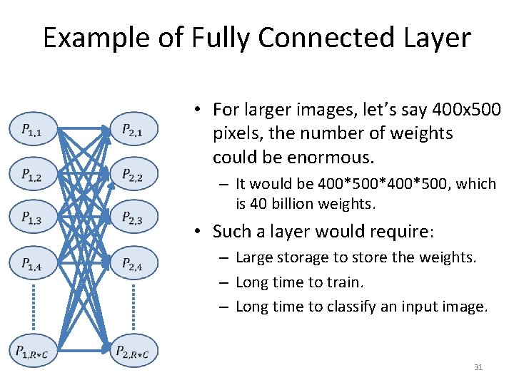
Example of Fully Connected Layer • For larger images, let’s say 400 x 500 pixels, the number of weights could be enormous. – It would be 400*500*400*500, which is 40 billion weights. • Such a layer would require: – Large storage to store the weights. – Long time to train. – Long time to classify an input image. 31

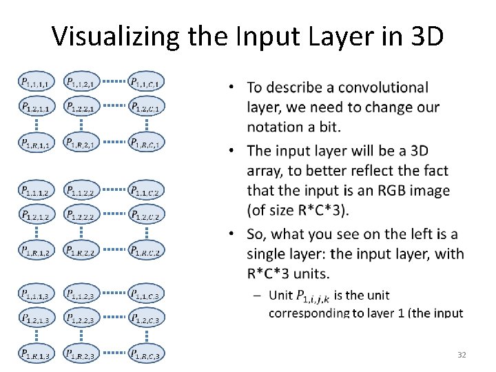
Visualizing the Input Layer in 3 D • 32

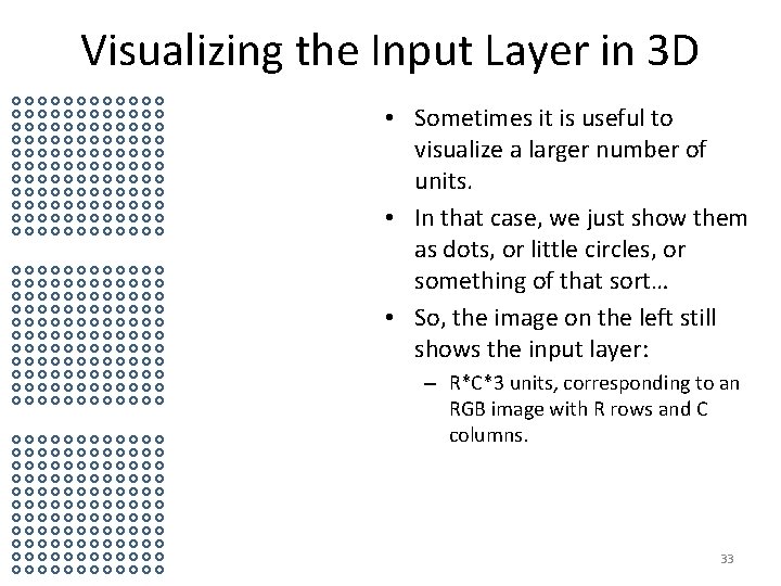
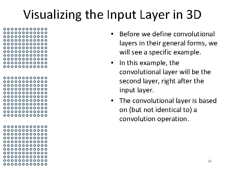
Visualizing the Input Layer in 3 D • Sometimes it is useful to visualize a larger number of units. • In that case, we just show them as dots, or little circles, or something of that sort… • So, the image on the left still shows the input layer: – R*C*3 units, corresponding to an RGB image with R rows and C columns. 33

Visualizing the Input Layer in 3 D • Before we define convolutional layers in their general forms, we will see a specific example. • In this example, the convolutional layer will be the second layer, right after the input layer. • The convolutional layer is based on (but not identical to) a convolution operation. 34

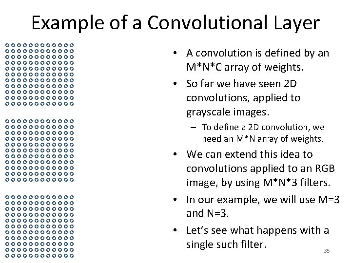
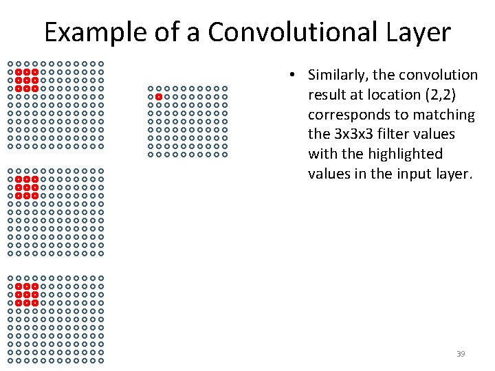
Example of a Convolutional Layer • A convolution is defined by an M*N*C array of weights. • So far we have seen 2 D convolutions, applied to grayscale images. – To define a 2 D convolution, we need an M*N array of weights. • We can extend this idea to convolutions applied to an RGB image, by using M*N*3 filters. • In our example, we will use M=3 and N=3. • Let’s see what happens with a single such filter. 35

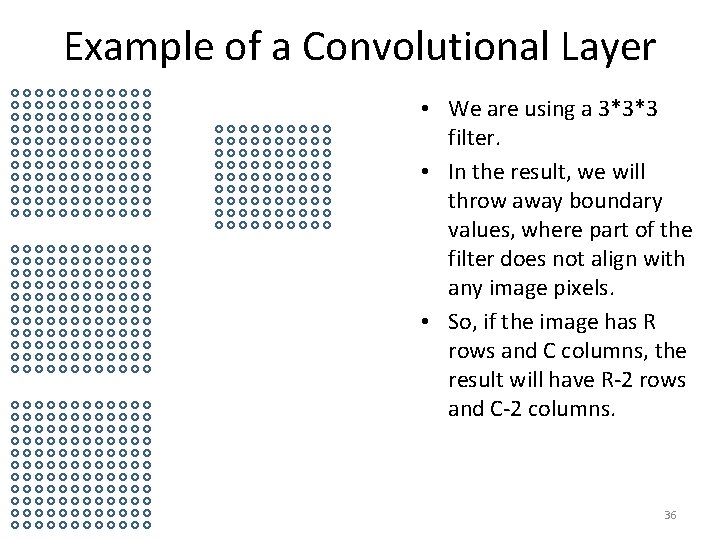
Example of a Convolutional Layer • We are using a 3*3*3 filter. • In the result, we will throw away boundary values, where part of the filter does not align with any image pixels. • So, if the image has R rows and C columns, the result will have R-2 rows and C-2 columns. 36

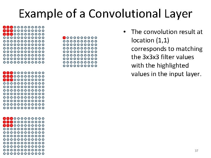
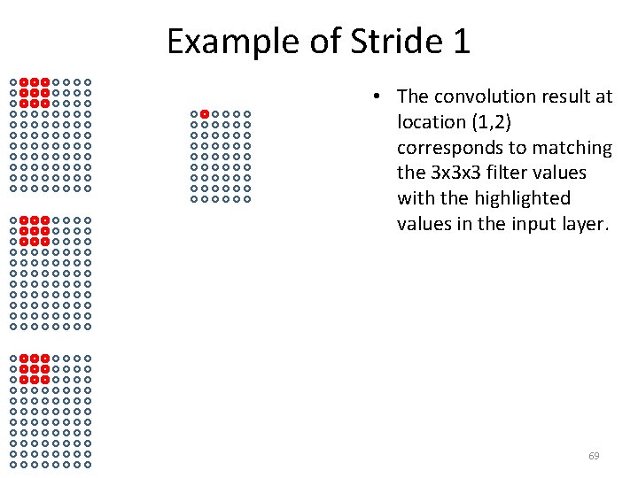
Example of a Convolutional Layer • The convolution result at location (1, 1) corresponds to matching the 3 x 3 x 3 filter values with the highlighted values in the input layer. 37

Example of a Convolutional Layer • Similarly, the convolution result at location (1, 2) corresponds to matching the 3 x 3 x 3 filter values with the highlighted values in the input layer. 38

Example of a Convolutional Layer • Similarly, the convolution result at location (2, 2) corresponds to matching the 3 x 3 x 3 filter values with the highlighted values in the input layer. 39

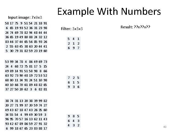
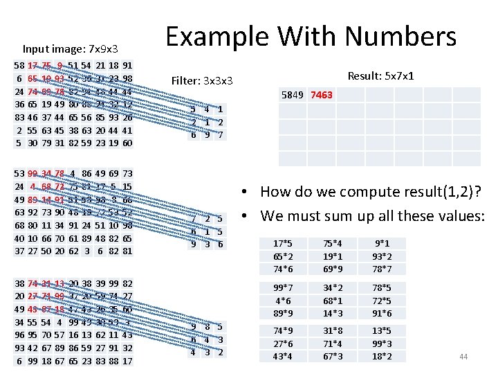
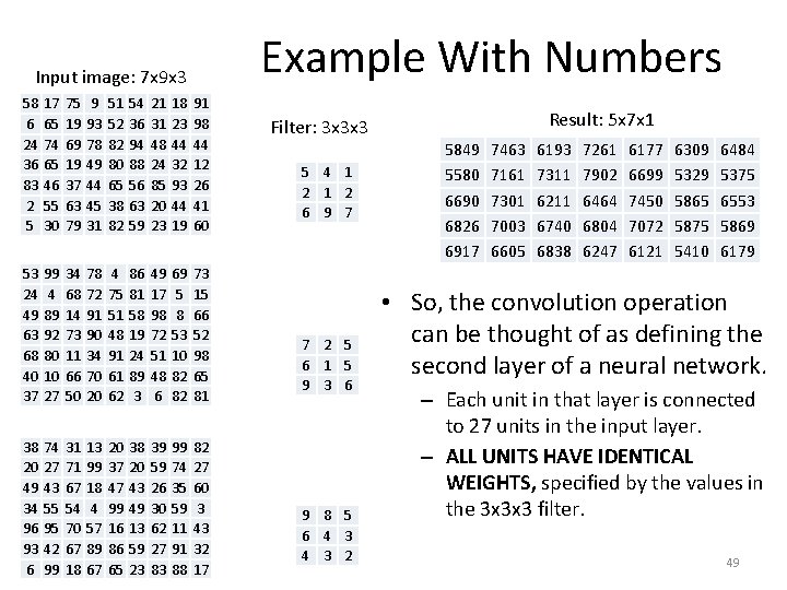
Example With Numbers Input image: 7 x 9 x 3 58 6 24 36 83 2 5 17 65 74 65 46 55 30 75 19 69 19 37 63 79 9 93 78 49 44 45 31 51 52 82 80 65 38 82 54 36 94 88 56 63 59 21 31 48 24 85 20 23 18 23 44 32 93 44 19 91 98 44 12 26 41 60 53 24 49 63 68 40 37 99 4 89 92 80 10 27 34 68 14 73 11 66 50 78 72 91 90 34 70 20 4 75 51 48 91 61 62 86 81 58 19 24 89 3 49 17 98 72 51 48 6 69 5 8 53 10 82 82 73 15 66 52 98 65 81 38 20 49 34 96 93 6 74 27 43 55 95 42 99 31 71 67 54 70 67 18 13 99 18 4 57 89 67 20 37 47 99 16 86 65 38 20 43 49 13 59 23 39 59 26 30 62 27 83 99 74 35 59 11 91 88 82 27 60 3 43 32 17 Filter: 3 x 3 x 3 Result: ? ? x? ? 5 4 1 2 6 9 7 7 2 5 6 1 5 9 3 6 9 8 5 6 4 3 2 40

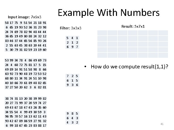
Example With Numbers Input image: 7 x 9 x 3 58 6 24 36 83 2 5 17 65 74 65 46 55 30 75 19 69 19 37 63 79 9 93 78 49 44 45 31 51 52 82 80 65 38 82 54 36 94 88 56 63 59 21 31 48 24 85 20 23 18 23 44 32 93 44 19 91 98 44 12 26 41 60 53 24 49 63 68 40 37 99 4 89 92 80 10 27 34 68 14 73 11 66 50 78 72 91 90 34 70 20 4 75 51 48 91 61 62 86 81 58 19 24 89 3 49 17 98 72 51 48 6 69 5 8 53 10 82 82 73 15 66 52 98 65 81 38 20 49 34 96 93 6 74 27 43 55 95 42 99 31 71 67 54 70 67 18 13 99 18 4 57 89 67 20 37 47 99 16 86 65 38 20 43 49 13 59 23 39 59 26 30 62 27 83 99 74 35 59 11 91 88 82 27 60 3 43 32 17 Filter: 3 x 3 x 3 Result: 5 x 7 x 1 5 4 1 2 6 9 7 • How do we compute result(1, 1)? 7 2 5 6 1 5 9 3 6 9 8 5 6 4 3 2 41

Example With Numbers Input image: 7 x 9 x 3 58 6 24 36 83 2 5 17 65 74 65 46 55 30 75 19 69 19 37 63 79 9 93 78 49 44 45 31 51 52 82 80 65 38 82 54 36 94 88 56 63 59 21 31 48 24 85 20 23 18 23 44 32 93 44 19 91 98 44 12 26 41 60 53 24 49 63 68 40 37 99 4 89 92 80 10 27 34 68 14 73 11 66 50 78 72 91 90 34 70 20 4 75 51 48 91 61 62 86 81 58 19 24 89 3 49 17 98 72 51 48 6 69 5 8 53 10 82 82 73 15 66 52 98 65 81 38 20 49 34 96 93 6 74 27 43 55 95 42 99 31 71 67 54 70 67 18 13 99 18 4 57 89 67 20 37 47 99 16 86 65 38 20 43 49 13 59 23 39 59 26 30 62 27 83 99 74 35 59 11 91 88 82 27 60 3 43 32 17 Filter: 3 x 3 x 3 Result: 5 x 7 x 1 5849 5 4 1 2 6 9 7 7 2 5 6 1 5 9 3 6 9 8 5 6 4 3 2 • How do we compute result(1, 1)? • We must sum up all these values: 58*5 6*2 24*6 17*4 65*1 74*9 75*1 19*2 69*7 53*7 24*6 49*9 99*2 4*1 89*3 34*5 68*5 14*6 38*9 20*6 49*4 74*8 27*4 43*3 31*5 71*3 67*2 42

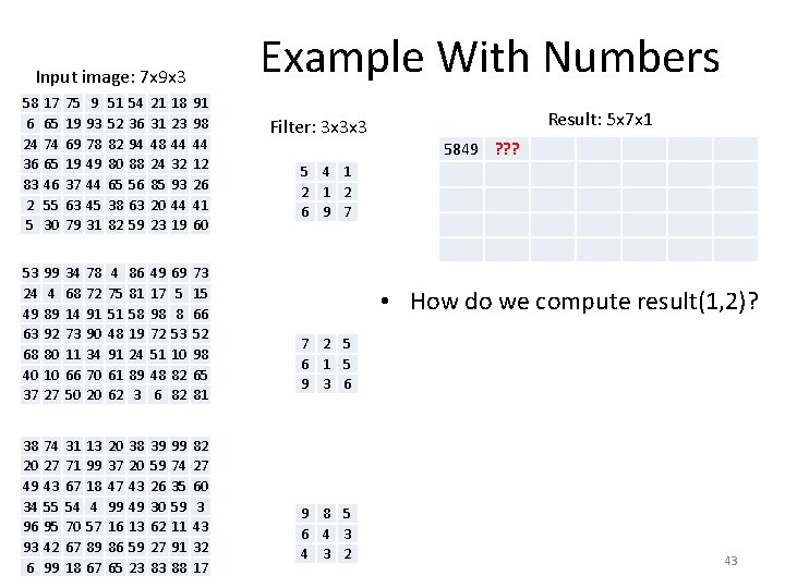
Example With Numbers Input image: 7 x 9 x 3 58 6 24 36 83 2 5 17 65 74 65 46 55 30 75 19 69 19 37 63 79 9 93 78 49 44 45 31 51 52 82 80 65 38 82 54 36 94 88 56 63 59 21 31 48 24 85 20 23 18 23 44 32 93 44 19 91 98 44 12 26 41 60 53 24 49 63 68 40 37 99 4 89 92 80 10 27 34 68 14 73 11 66 50 78 72 91 90 34 70 20 4 75 51 48 91 61 62 86 81 58 19 24 89 3 49 17 98 72 51 48 6 69 5 8 53 10 82 82 73 15 66 52 98 65 81 38 20 49 34 96 93 6 74 27 43 55 95 42 99 31 71 67 54 70 67 18 13 99 18 4 57 89 67 20 37 47 99 16 86 65 38 20 43 49 13 59 23 39 59 26 30 62 27 83 99 74 35 59 11 91 88 82 27 60 3 43 32 17 Filter: 3 x 3 x 3 Result: 5 x 7 x 1 5849 ? ? ? 5 4 1 2 6 9 7 • How do we compute result(1, 2)? 7 2 5 6 1 5 9 3 6 9 8 5 6 4 3 2 43

Example With Numbers Input image: 7 x 9 x 3 58 6 24 36 83 2 5 17 65 74 65 46 55 30 75 19 69 19 37 63 79 9 93 78 49 44 45 31 51 52 82 80 65 38 82 54 36 94 88 56 63 59 21 31 48 24 85 20 23 18 23 44 32 93 44 19 91 98 44 12 26 41 60 53 24 49 63 68 40 37 99 4 89 92 80 10 27 34 68 14 73 11 66 50 78 72 91 90 34 70 20 4 75 51 48 91 61 62 86 81 58 19 24 89 3 49 17 98 72 51 48 6 69 5 8 53 10 82 82 73 15 66 52 98 65 81 38 20 49 34 96 93 6 74 27 43 55 95 42 99 31 71 67 54 70 67 18 13 99 18 4 57 89 67 20 37 47 99 16 86 65 38 20 43 49 13 59 23 39 59 26 30 62 27 83 99 74 35 59 11 91 88 82 27 60 3 43 32 17 Filter: 3 x 3 x 3 Result: 5 x 7 x 1 5849 7463 5 4 1 2 6 9 7 7 2 5 6 1 5 9 3 6 9 8 5 6 4 3 2 • How do we compute result(1, 2)? • We must sum up all these values: 17*5 65*2 74*6 75*4 19*1 69*9 9*1 93*2 78*7 99*7 4*6 89*9 34*2 68*1 14*3 78*5 72*5 91*6 74*9 27*6 43*4 31*8 71*4 67*3 13*5 99*3 18*2 44

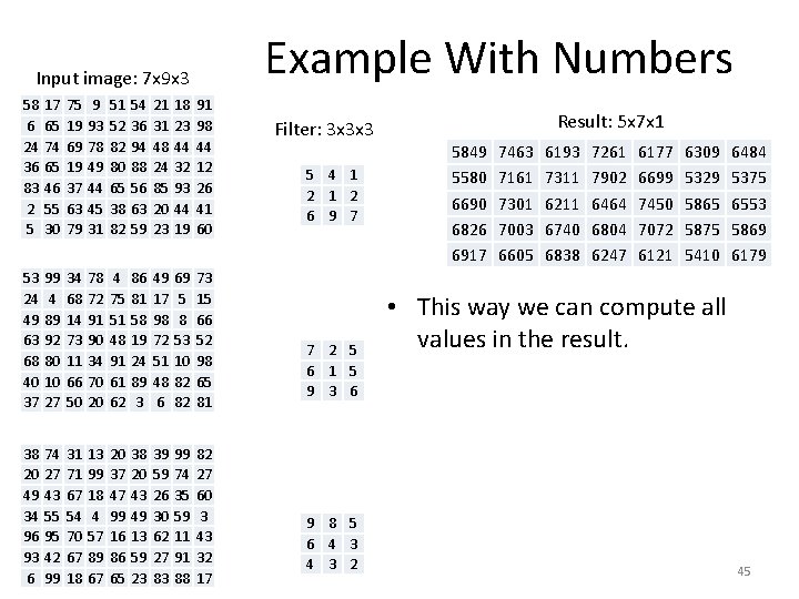
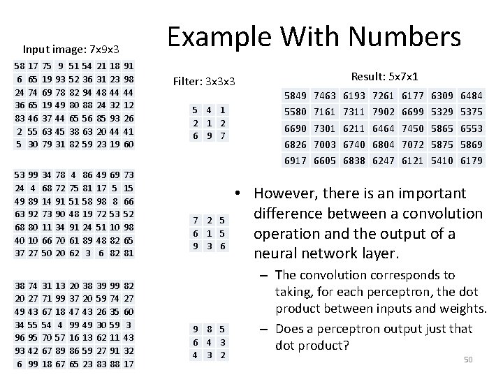
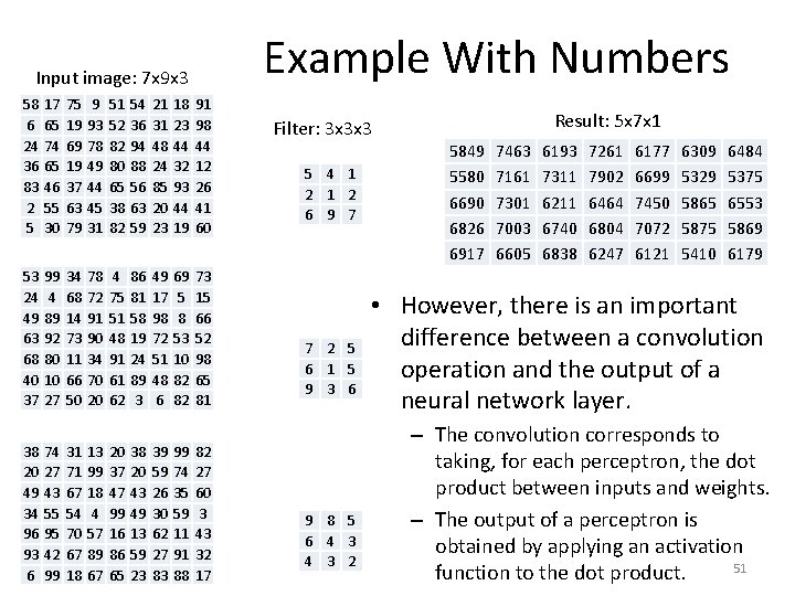
Example With Numbers Input image: 7 x 9 x 3 58 6 24 36 83 2 5 17 65 74 65 46 55 30 75 19 69 19 37 63 79 9 93 78 49 44 45 31 51 52 82 80 65 38 82 54 36 94 88 56 63 59 21 31 48 24 85 20 23 18 23 44 32 93 44 19 91 98 44 12 26 41 60 53 24 49 63 68 40 37 99 4 89 92 80 10 27 34 68 14 73 11 66 50 78 72 91 90 34 70 20 4 75 51 48 91 61 62 86 81 58 19 24 89 3 49 17 98 72 51 48 6 69 5 8 53 10 82 82 73 15 66 52 98 65 81 38 20 49 34 96 93 6 74 27 43 55 95 42 99 31 71 67 54 70 67 18 13 99 18 4 57 89 67 20 37 47 99 16 86 65 38 20 43 49 13 59 23 39 59 26 30 62 27 83 99 74 35 59 11 91 88 82 27 60 3 43 32 17 Filter: 3 x 3 x 3 5 4 1 2 6 9 7 7 2 5 6 1 5 9 3 6 9 8 5 6 4 3 2 Result: 5 x 7 x 1 5849 5580 6690 6826 6917 7463 7161 7301 7003 6605 6193 7311 6211 6740 6838 7261 7902 6464 6804 6247 6177 6699 7450 7072 6121 6309 5329 5865 5875 5410 6484 5375 6553 5869 6179 • This way we can compute all values in the result. 45

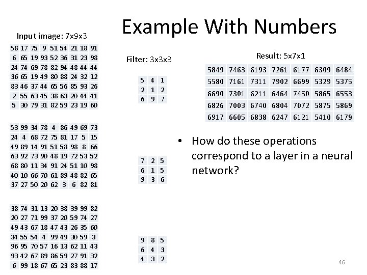
Example With Numbers Input image: 7 x 9 x 3 58 6 24 36 83 2 5 17 65 74 65 46 55 30 75 19 69 19 37 63 79 9 93 78 49 44 45 31 51 52 82 80 65 38 82 54 36 94 88 56 63 59 21 31 48 24 85 20 23 18 23 44 32 93 44 19 91 98 44 12 26 41 60 53 24 49 63 68 40 37 99 4 89 92 80 10 27 34 68 14 73 11 66 50 78 72 91 90 34 70 20 4 75 51 48 91 61 62 86 81 58 19 24 89 3 49 17 98 72 51 48 6 69 5 8 53 10 82 82 73 15 66 52 98 65 81 38 20 49 34 96 93 6 74 27 43 55 95 42 99 31 71 67 54 70 67 18 13 99 18 4 57 89 67 20 37 47 99 16 86 65 38 20 43 49 13 59 23 39 59 26 30 62 27 83 99 74 35 59 11 91 88 82 27 60 3 43 32 17 Filter: 3 x 3 x 3 5 4 1 2 6 9 7 7 2 5 6 1 5 9 3 6 9 8 5 6 4 3 2 Result: 5 x 7 x 1 5849 5580 6690 6826 6917 7463 7161 7301 7003 6605 6193 7311 6211 6740 6838 7261 7902 6464 6804 6247 6177 6699 7450 7072 6121 6309 5329 5865 5875 5410 6484 5375 6553 5869 6179 • How do these operations correspond to a layer in a neural network? 46

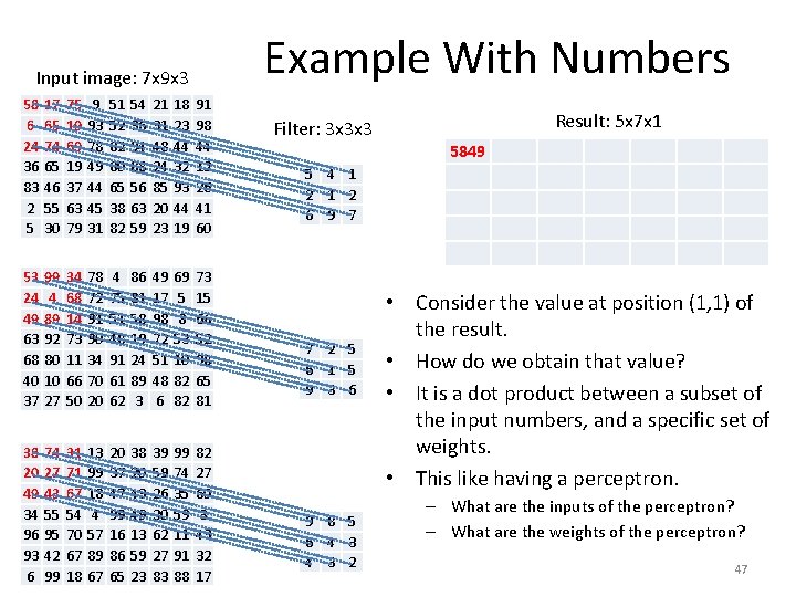
Example With Numbers Input image: 7 x 9 x 3 58 6 24 36 83 2 5 17 65 74 65 46 55 30 75 19 69 19 37 63 79 9 93 78 49 44 45 31 51 52 82 80 65 38 82 54 36 94 88 56 63 59 21 31 48 24 85 20 23 18 23 44 32 93 44 19 91 98 44 12 26 41 60 53 24 49 63 68 40 37 99 4 89 92 80 10 27 34 68 14 73 11 66 50 78 72 91 90 34 70 20 4 75 51 48 91 61 62 86 81 58 19 24 89 3 49 17 98 72 51 48 6 69 5 8 53 10 82 82 73 15 66 52 98 65 81 38 20 49 34 96 93 6 74 27 43 55 95 42 99 31 71 67 54 70 67 18 13 99 18 4 57 89 67 20 37 47 99 16 86 65 38 20 43 49 13 59 23 39 59 26 30 62 27 83 99 74 35 59 11 91 88 82 27 60 3 43 32 17 Filter: 3 x 3 x 3 Result: 5 x 7 x 1 5849 5 4 1 2 6 9 7 7 2 5 6 1 5 9 3 6 9 8 5 6 4 3 2 • Consider the value at position (1, 1) of the result. • How do we obtain that value? • It is a dot product between a subset of the input numbers, and a specific set of weights. • This like having a perceptron. – What are the inputs of the perceptron? – What are the weights of the perceptron? 47

Example With Numbers Input image: 7 x 9 x 3 58 6 24 36 83 2 5 17 65 74 65 46 55 30 75 19 69 19 37 63 79 9 93 78 49 44 45 31 51 52 82 80 65 38 82 54 36 94 88 56 63 59 21 31 48 24 85 20 23 18 23 44 32 93 44 19 91 98 44 12 26 41 60 53 24 49 63 68 40 37 99 4 89 92 80 10 27 34 68 14 73 11 66 50 78 72 91 90 34 70 20 4 75 51 48 91 61 62 86 81 58 19 24 89 3 49 17 98 72 51 48 6 69 5 8 53 10 82 82 73 15 66 52 98 65 81 38 20 49 34 96 93 6 74 27 43 55 95 42 99 31 71 67 54 70 67 18 13 99 18 4 57 89 67 20 37 47 99 16 86 65 38 20 43 49 13 59 23 39 59 26 30 62 27 83 99 74 35 59 11 91 88 82 27 60 3 43 32 17 Filter: 3 x 3 x 3 Result: 5 x 7 x 1 5849 5 4 1 2 6 9 7 7 2 5 6 1 5 9 3 6 9 8 5 6 4 3 2 • Consider the value at position (1, 1) of the result. • How do we obtain that value? • It is a dot product between a subset of the input numbers, and a specific set of weights. • This like having a perceptron. – Perceptron inputs are the red values – Perceptron weights are the filter values. 48

Example With Numbers Input image: 7 x 9 x 3 58 6 24 36 83 2 5 17 65 74 65 46 55 30 75 19 69 19 37 63 79 9 93 78 49 44 45 31 51 52 82 80 65 38 82 54 36 94 88 56 63 59 21 31 48 24 85 20 23 18 23 44 32 93 44 19 91 98 44 12 26 41 60 53 24 49 63 68 40 37 99 4 89 92 80 10 27 34 68 14 73 11 66 50 78 72 91 90 34 70 20 4 75 51 48 91 61 62 86 81 58 19 24 89 3 49 17 98 72 51 48 6 69 5 8 53 10 82 82 73 15 66 52 98 65 81 38 20 49 34 96 93 6 74 27 43 55 95 42 99 31 71 67 54 70 67 18 13 99 18 4 57 89 67 20 37 47 99 16 86 65 38 20 43 49 13 59 23 39 59 26 30 62 27 83 99 74 35 59 11 91 88 82 27 60 3 43 32 17 Filter: 3 x 3 x 3 5 4 1 2 6 9 7 7 2 5 6 1 5 9 3 6 9 8 5 6 4 3 2 Result: 5 x 7 x 1 5849 5580 6690 6826 6917 7463 7161 7301 7003 6605 6193 7311 6211 6740 6838 7261 7902 6464 6804 6247 6177 6699 7450 7072 6121 6309 5329 5865 5875 5410 6484 5375 6553 5869 6179 • So, the convolution operation can be thought of as defining the second layer of a neural network. – Each unit in that layer is connected to 27 units in the input layer. – ALL UNITS HAVE IDENTICAL WEIGHTS, specified by the values in the 3 x 3 x 3 filter. 49

Example With Numbers Input image: 7 x 9 x 3 58 6 24 36 83 2 5 17 65 74 65 46 55 30 75 19 69 19 37 63 79 9 93 78 49 44 45 31 51 52 82 80 65 38 82 54 36 94 88 56 63 59 21 31 48 24 85 20 23 18 23 44 32 93 44 19 91 98 44 12 26 41 60 53 24 49 63 68 40 37 99 4 89 92 80 10 27 34 68 14 73 11 66 50 78 72 91 90 34 70 20 4 75 51 48 91 61 62 86 81 58 19 24 89 3 49 17 98 72 51 48 6 69 5 8 53 10 82 82 73 15 66 52 98 65 81 38 20 49 34 96 93 6 74 27 43 55 95 42 99 31 71 67 54 70 67 18 13 99 18 4 57 89 67 20 37 47 99 16 86 65 38 20 43 49 13 59 23 39 59 26 30 62 27 83 99 74 35 59 11 91 88 82 27 60 3 43 32 17 Filter: 3 x 3 x 3 5 4 1 2 6 9 7 7 2 5 6 1 5 9 3 6 9 8 5 6 4 3 2 Result: 5 x 7 x 1 5849 5580 6690 6826 6917 7463 7161 7301 7003 6605 6193 7311 6211 6740 6838 7261 7902 6464 6804 6247 6177 6699 7450 7072 6121 6309 5329 5865 5875 5410 6484 5375 6553 5869 6179 • However, there is an important difference between a convolution operation and the output of a neural network layer. – The convolution corresponds to taking, for each perceptron, the dot product between inputs and weights. – Does a perceptron output just that dot product? 50

Example With Numbers Input image: 7 x 9 x 3 58 6 24 36 83 2 5 17 65 74 65 46 55 30 75 19 69 19 37 63 79 9 93 78 49 44 45 31 51 52 82 80 65 38 82 54 36 94 88 56 63 59 21 31 48 24 85 20 23 18 23 44 32 93 44 19 91 98 44 12 26 41 60 53 24 49 63 68 40 37 99 4 89 92 80 10 27 34 68 14 73 11 66 50 78 72 91 90 34 70 20 4 75 51 48 91 61 62 86 81 58 19 24 89 3 49 17 98 72 51 48 6 69 5 8 53 10 82 82 73 15 66 52 98 65 81 38 20 49 34 96 93 6 74 27 43 55 95 42 99 31 71 67 54 70 67 18 13 99 18 4 57 89 67 20 37 47 99 16 86 65 38 20 43 49 13 59 23 39 59 26 30 62 27 83 99 74 35 59 11 91 88 82 27 60 3 43 32 17 Filter: 3 x 3 x 3 5 4 1 2 6 9 7 7 2 5 6 1 5 9 3 6 9 8 5 6 4 3 2 Result: 5 x 7 x 1 5849 5580 6690 6826 6917 7463 7161 7301 7003 6605 6193 7311 6211 6740 6838 7261 7902 6464 6804 6247 6177 6699 7450 7072 6121 6309 5329 5865 5875 5410 6484 5375 6553 5869 6179 • However, there is an important difference between a convolution operation and the output of a neural network layer. – The convolution corresponds to taking, for each perceptron, the dot product between inputs and weights. – The output of a perceptron is obtained by applying an activation 51 function to the dot product.

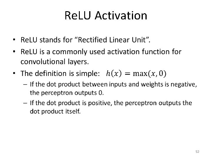
Re. LU Activation • 52

Convolutional Layers • So, a convolution can be thought of as specifying a neural network layer. • The filter values specify the weights of every single perceptron in the layer. • However, remember that the output of a convolutional layer is not the result of the convolution. – Each dot product passes through an activation function (usually Re. LU) in order to produce an output. 53

Applying Multiple Convolutions • In our previous example: – We started with a 3 -channel input image (an RGB image). • This defined a 3 D array of input units, of dimensions R*C*3. – We applied a single 3 x 3 x 3 convolutional filter. – We obtained a 1 -channel output. • This defined a 2 D array of units in the convolutional layer. • We can apply multiple convolutions at the same time. – We can apply K different 3 x 3 x 3 convolutional filters. – This leads to a K-channel output. • This defines a 3 D array of units in the convolutional layer, of dimensions (R-2)*(C-2)*K. • Each 2 D slice of that array corresponds to a single 3 x 3 x 3 filter. 54

Example of Multiple Convolutions • In our previous example: – We started with a 3 -channel input image (an RGB image). • This defined a 3 D array of input units, of dimensions R*C*3. – We applied a single 3 x 3 x 3 convolutional filter. – We obtained a 1 -channel output. • This defined a 2 D array of units in the convolutional layer. • We can apply multiple convolutions at the same time. – We can apply K different 3 x 3 x 3 convolutional filters. – This leads to a K-channel output. • This defines a 3 D array of units in the convolutional layer, of dimensions (R-2)*(C-2)*K. • Each 2 D slice of that array corresponds to a single 3 x 3 x 3 filter. 55

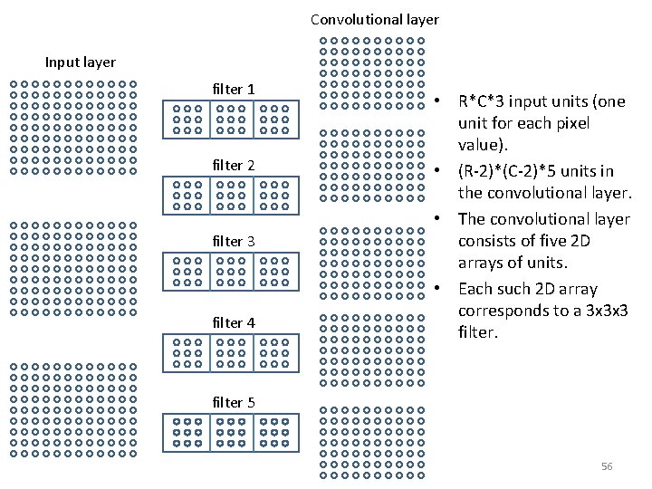
Convolutional layer Input layer filter 1 filter 2 filter 3 filter 4 • R*C*3 input units (one unit for each pixel value). • (R-2)*(C-2)*5 units in the convolutional layer. • The convolutional layer consists of five 2 D arrays of units. • Each such 2 D array corresponds to a 3 x 3 x 3 filter 5 56

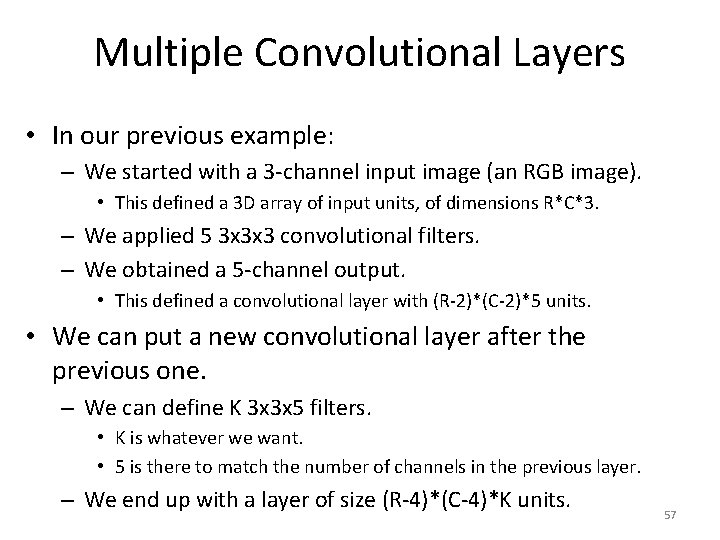
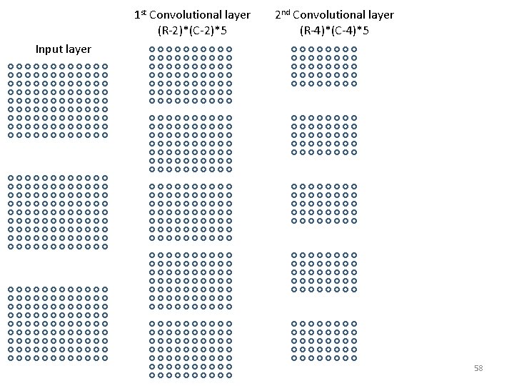
Multiple Convolutional Layers • In our previous example: – We started with a 3 -channel input image (an RGB image). • This defined a 3 D array of input units, of dimensions R*C*3. – We applied 5 3 x 3 x 3 convolutional filters. – We obtained a 5 -channel output. • This defined a convolutional layer with (R-2)*(C-2)*5 units. • We can put a new convolutional layer after the previous one. – We can define K 3 x 3 x 5 filters. • K is whatever we want. • 5 is there to match the number of channels in the previous layer. – We end up with a layer of size (R-4)*(C-4)*K units. 57

1 st Convolutional layer (R-2)*(C-2)*5 2 nd Convolutional layer (R-4)*(C-4)*5 Input layer 58

Multiple Convolutional Layers • Overall, we can put as many convolutional layers in sequence as we want. 59

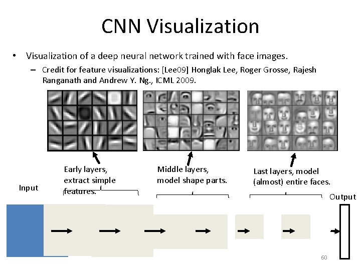
CNN Visualization • Visualization of a deep neural network trained with face images. – Credit for feature visualizations: [Lee 09] Honglak Lee, Roger Grosse, Rajesh Ranganath and Andrew Y. Ng. , ICML 2009. Input Early layers, extract simple features. Middle layers, model shape parts. Last layers, model (almost) entire faces. Output 60

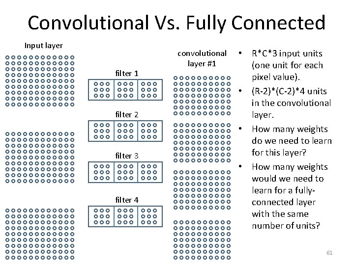
Convolutional Vs. Fully Connected Input layer filter 1 filter 2 filter 3 filter 4 convolutional layer #1 • R*C*3 input units (one unit for each pixel value). • (R-2)*(C-2)*4 units in the convolutional layer. • How many weights do we need to learn for this layer? • How many weights would we need to learn for a fullyconnected layer with the same number of units? 61

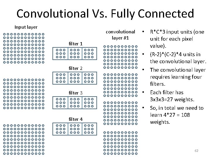
Convolutional Vs. Fully Connected Input layer filter 1 filter 2 filter 3 filter 4 convolutional layer #1 • R*C*3 input units (one unit for each pixel value). • (R-2)*(C-2)*4 units in the convolutional layer. • The convolutional layer requires learning four filters. • Each filter has 3 x 3 x 3=27 weights. • So, in total we need to learn 4*27 = 108 weights. 62

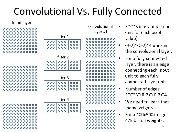
Convolutional Vs. Fully Connected Input layer filter 1 filter 2 filter 3 filter 4 convolutional layer #1 • R*C*3 input units (one unit for each pixel value). • (R-2)*(C-2)*4 units in the convolutional layer. • For a fully connected layer, there is an edge connecting each input unit to each fully connected layer unit. • Number of edges: R*C*3*(R-2)*(C-2)*4. • We need to learn that many weights. • For a 400 x 500 image: 475 billion weights. 63

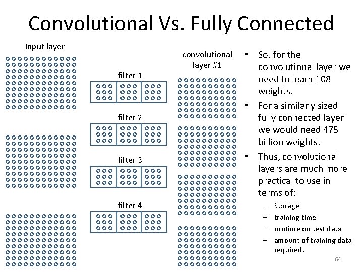
Convolutional Vs. Fully Connected Input layer filter 1 filter 2 filter 3 filter 4 convolutional layer #1 • So, for the convolutional layer we need to learn 108 weights. • For a similarly sized fully connected layer we would need 475 billion weights. • Thus, convolutional layers are much more practical to use in terms of: – – Storage training time runtime on test data amount of training data required. 64

Max Pooling Layer • A max pooling layer is a layer where every unit corresponds to a 2 x 2 (or 3 x 3) neighborhood in the previous layer, and the output is the maximum value in that neighborhood. 65

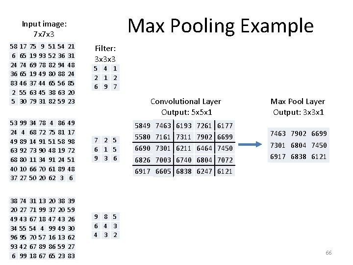
Max Pooling Example Input image: 7 x 7 x 3 58 6 24 36 83 2 5 17 65 74 65 46 55 30 75 19 69 19 37 63 79 9 93 78 49 44 45 31 51 52 82 80 65 38 82 54 36 94 88 56 63 59 21 31 48 24 85 20 23 53 24 49 63 68 40 37 99 4 89 92 80 10 27 34 68 14 73 11 66 50 78 72 91 90 34 70 20 4 75 51 48 91 61 62 86 81 58 19 24 89 3 49 17 98 72 51 48 6 7 2 5 6 1 5 9 3 6 38 20 49 34 96 93 6 74 27 43 55 95 42 99 31 71 67 54 70 67 18 13 99 18 4 57 89 67 20 37 47 99 16 86 65 38 20 43 49 13 59 23 39 59 26 30 62 27 83 9 8 5 6 4 3 2 Filter: 3 x 3 x 3 5 4 1 2 6 9 7 Convolutional Layer Output: 5 x 5 x 1 5849 5580 6690 6826 6917 7463 7161 7301 7003 6605 6193 7311 6211 6740 6838 7261 7902 6464 6804 6247 6177 6699 7450 7072 6121 Max Pool Layer Output: 3 x 3 x 1 7463 7902 6699 7301 6804 7450 6917 6838 6121 66

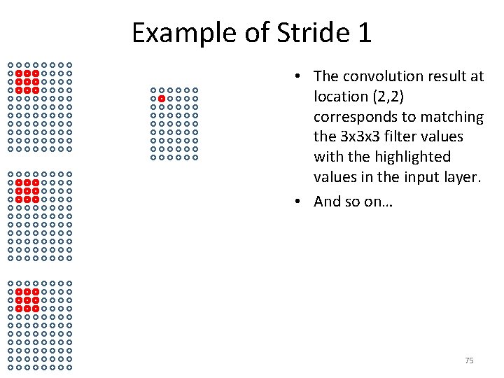
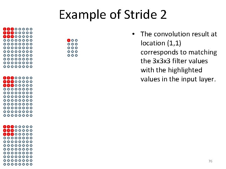
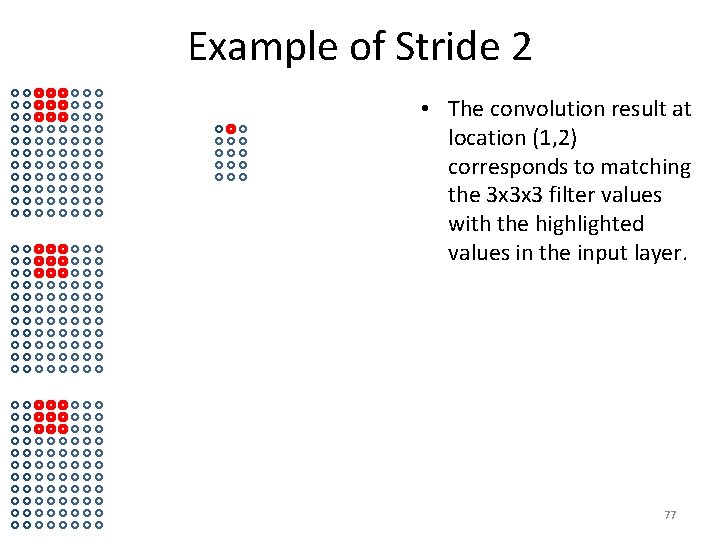
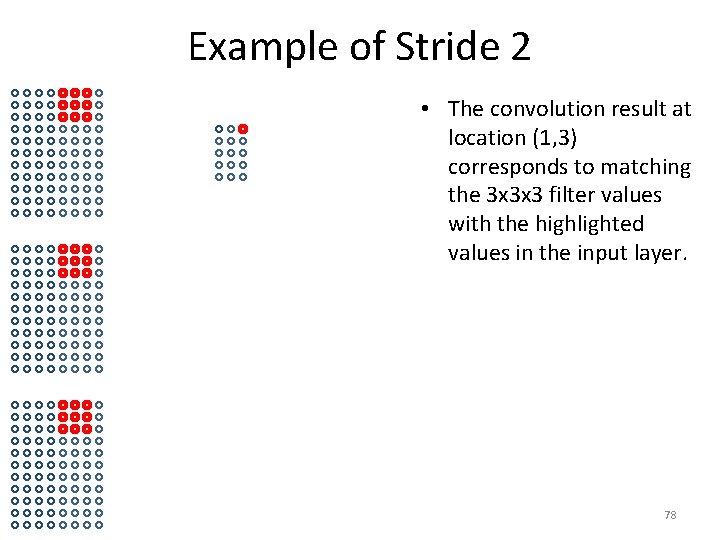
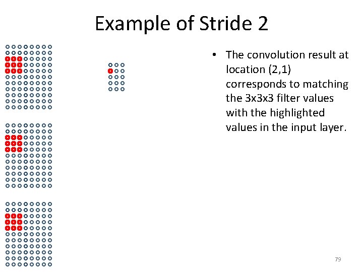
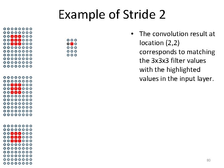
Stride • For each convolutional layer, we can pick a stride S. • S is a single number, that influences the number of outputs of the convolutional layer. – It determines how many locations to shift the filter to the left or to the bottom to compute the next value of the convolution result. • Stride = 1: we shift the filter one location at a time, so no rows or columns are skipped. • Stride = 2: we shift the filter two locations at a time. Half the rows and half the columns are skipped. – This means that the convolutional layer will have about half the number of rows and columns of the previous layer. 67

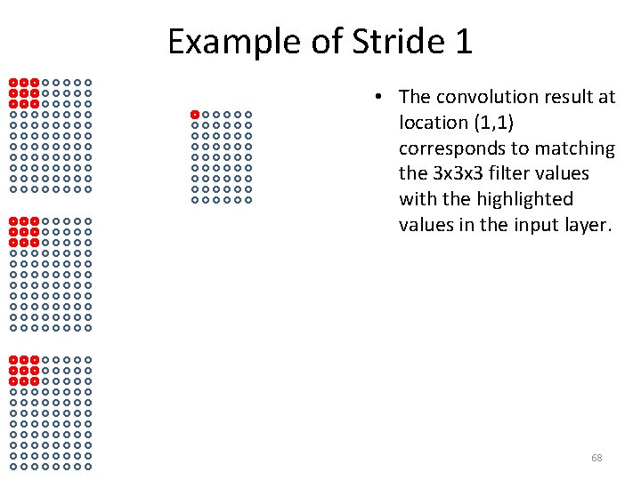
Example of Stride 1 • The convolution result at location (1, 1) corresponds to matching the 3 x 3 x 3 filter values with the highlighted values in the input layer. 68

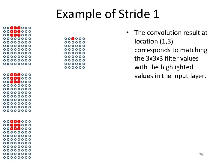
Example of Stride 1 • The convolution result at location (1, 2) corresponds to matching the 3 x 3 x 3 filter values with the highlighted values in the input layer. 69

Example of Stride 1 • The convolution result at location (1, 3) corresponds to matching the 3 x 3 x 3 filter values with the highlighted values in the input layer. 70

Example of Stride 1 • The convolution result at location (1, 4) corresponds to matching the 3 x 3 x 3 filter values with the highlighted values in the input layer. 71

Example of Stride 1 • The convolution result at location (1, 5) corresponds to matching the 3 x 3 x 3 filter values with the highlighted values in the input layer. 72

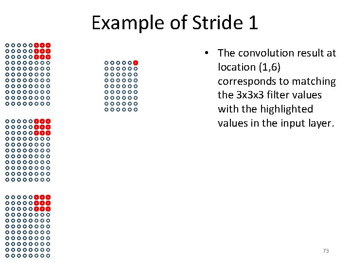
Example of Stride 1 • The convolution result at location (1, 6) corresponds to matching the 3 x 3 x 3 filter values with the highlighted values in the input layer. 73

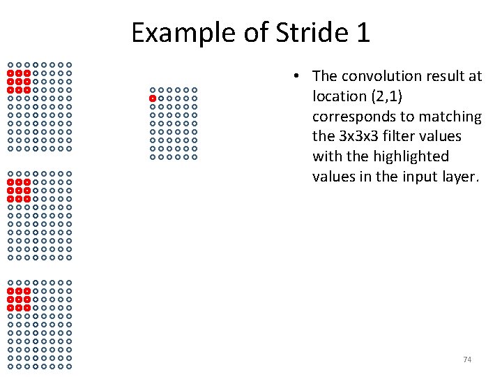
Example of Stride 1 • The convolution result at location (2, 1) corresponds to matching the 3 x 3 x 3 filter values with the highlighted values in the input layer. 74

Example of Stride 1 • The convolution result at location (2, 2) corresponds to matching the 3 x 3 x 3 filter values with the highlighted values in the input layer. • And so on… 75

Example of Stride 2 • The convolution result at location (1, 1) corresponds to matching the 3 x 3 x 3 filter values with the highlighted values in the input layer. 76

Example of Stride 2 • The convolution result at location (1, 2) corresponds to matching the 3 x 3 x 3 filter values with the highlighted values in the input layer. 77

Example of Stride 2 • The convolution result at location (1, 3) corresponds to matching the 3 x 3 x 3 filter values with the highlighted values in the input layer. 78

Example of Stride 2 • The convolution result at location (2, 1) corresponds to matching the 3 x 3 x 3 filter values with the highlighted values in the input layer. 79

Example of Stride 2 • The convolution result at location (2, 2) corresponds to matching the 3 x 3 x 3 filter values with the highlighted values in the input layer. 80

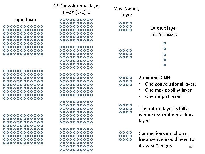
Fully Connected Output Layer • The output layer has as many units as the number of classes. • The layer preceding the output layer is called the last hidden layer. • Usually the output layer is fully connected to its previous layer. – “Fully connected” means that all units in the output layer take as input all outputs of the last hidden layer. • The last hidden layer can be a convolutional layer or a max pooling layer. 81

1 st Convolutional layer (R-2)*(C-2)*5 Input layer Max Pooling Layer Output layer for 5 classes A minimal CNN • One convolutional layer. • One max pooling layer • One output layer. The output layer is fully connected to the previous layer. Connections not shown because we would need to draw 300 edges. 82

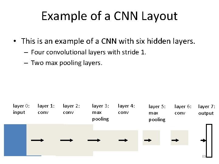
Example of a CNN Layout • This is an example of a CNN with six hidden layers. – Four convolutional layers with stride 1. – Two max pooling layers. layer 0: input layer 1: conv layer 2: conv layer 3: max pooling layer 4: conv layer 5: max pooling layer 6: conv layer 7: output 83

Transfer Learning • Image. Net is a public dataset has over 14 million images, over 20, 000 classes (such as “balloon” or “strawberry”). – http: //www. image-net. org/ – https: //en. wikipedia. org/wiki/Image. Net • CNNs can be (and have been) trained on such large datasets. • Suppose that you have some training images of three animals that were recently discovered. – Let’s say, 100 images for each animal. – You want a classifier that recognizes each of the two animals. • Is the Image. Net data useful? – Image. Net does not contain images of those two animals. 84

Transfer Learning • Simple approach: train a classifier on your 300 images. • 300 images is a rather small dataset, so you would use a relatively simple model. – Complicated models would probably overfit. – At the same time, a simple model would probably have limited accuracy. 85

Transfer Learning • Transfer learning approach: – 1 st step: train a CNN on Image. Net. • Actually, these days you can just download a pre-trained model, so you do not have to do the training yourself. – 2 nd step: throw away the output layer of the CNN. • The last layer recognizes Image. Net classes, which you don’t care about. – 3 rd step: create a new output layer with three units, and connect it to the last hidden layer of the pre-trained CNN. – 4 th step: train just the weights of the new output layer with your new dataset. 86

Transfer Learning • Why is it called “transfer learning”? – Because, in order to learn a classifier for our three animals, we are transferring information learned from training examples (Image. Net) that did not include those three animals. – So, to recognize some classes, we use (partly) training examples from other classes. • What information are we transferring? – All the layers and weights of the Image. Net-trained model, except for the output layer. 87

Transfer Learning • Why would transfer learning be useful? • The last hidden layer of the pre-trained model is used to recognize over 20, 000 classes. • Presumably, that last hidden layer computes features that are useful for recognizing a very wide variety of visual objects and shapes. • Those features have been optimized using millions of training examples. • Transfer learning assumes that those features would be useful for our three animals as well. 88

Transfer Learning • Overall, we have a trade-off: • 1 st choice: Learn a model from scratch, using our three hundred images. – The model will be optimized exclusively for the three animals we want to recognize. – However, it will be a simple model, trained on a small training set. • 2 nd choice: Transfer learning. – Most of the model is optimized using examples that do not contain our three animals. – However, the features extracted by that model have been heavily optimized, and may be more useful than what we can learn from just 300 examples. 89

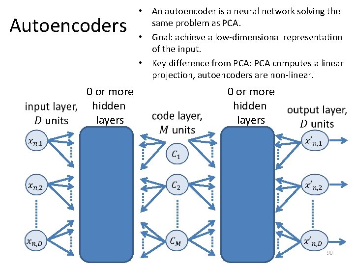
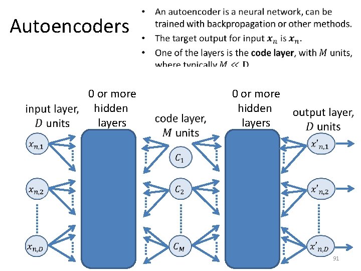
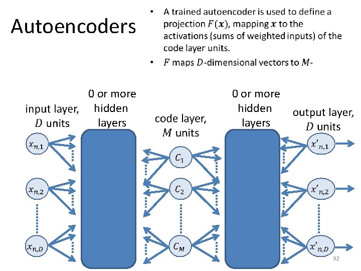
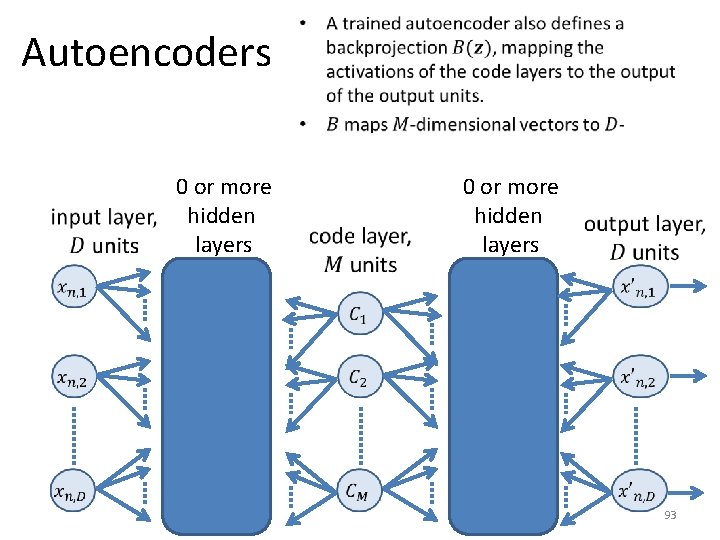
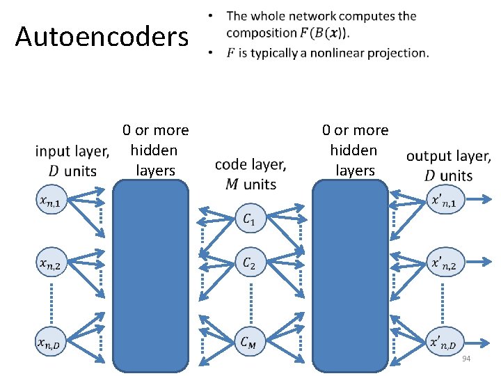
Autoencoders 0 or more hidden layers • An autoencoder is a neural network solving the same problem as PCA. • Goal: achieve a low-dimensional representation of the input. • Key difference from PCA: PCA computes a linear projection, autoencoders are non-linear. 0 or more hidden layers 90

Autoencoders 0 or more hidden layers • 0 or more hidden layers 91

Autoencoders 0 or more hidden layers • 0 or more hidden layers 92

Autoencoders 0 or more hidden layers • 0 or more hidden layers 93

Autoencoders 0 or more hidden layers • 0 or more hidden layers 94