Geographic Data and Relationships Outline Types of Geographic

Geographic Data and Relationships

Outline • Types of Geographic Data – spatial data – tabular data – image data • Acquiring Data • Storing Geographical data • Spatial Data Models and Structures – Vector data model • spaghetti • topological data structures (concepts of topology) – Raster data model – Database Structures • Referencing Spatial Data and Map Projections

Types of Geographic Data • Geographic data: data that describes any part of the Earth's surface or the features found on it such as: cartographic data, scientific data, business data, land records, photographs, customer databases, travel guides, real estate listings, legal documents, videos, etc. • Arc. View supports three types: – Spatial data. – Images. – Tabular (Descriptive) data.

Data Types Supported by Arc. GIS

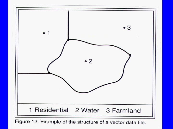
Spatial Data • Spatial data is geographic data that stores the geometric location of particular features, along with attribute information describing what these features represent. Also known as a digital map. – location data is stored in a vector or raster data structure. – Corresponding attribute data is stored in a set of tables related geographically to the features they describe. – Location, shape, tables, and the rest of the attributes together form what we call “spatial data”

Example of vector on raster data

Example of tabular data (attributes of measured highways)

Attributes of “Cities” in the “Topography” Data Frame

Spatial Data Format Supported by Arc. View • • • Arc. View shapefiles ARC/INFO coverages ARC/INFO GRID data Image data CAD drawings SDE data (If Database Access is installed) Street. Map data (If Street. Map is installed) TINs (If 3 D Analyst is installed) VPF data

Example of themes imported from Auto. Cad by “Cad Reader” in Arc. View

Differences between Spatial Data and Simple Vector Graphics or Images What is the difference between spatial data and a scanned image or a CAD file? ? 1 - In spatial data there is an explicit relationship between the geometric and attribute information, so that both are always available when you work with the data. For example, if you select particular features displayed on a view. Arc. View will automatically highlight the records containing the attributes of these features when the attribute table is displayed.

Streets selected on the map of SF are also selected in the table

2 - Spatial data is georeferenced to known locations on the Earth's surface. Coordinates 3 - Spatial data is organized thematically into different layers, or themes. There is one theme for each set of geographic features or phenomena for which information will be recorded. For example, streams, land use, elevation, and buildings will each be stored as a separate spatial data sources, rather than trying to store them all together in one layer.

4 - Spatial data is primarily feature based. It is designed to enable specific geographic features and phenomena to be managed, manipulated analyzed easily and flexibly.

1 - Vector Data • Usually constructed by digitizing a map or a photograph. • Features are represented by pairs of Cartesian coordinates. They can be points, lines, or polygons. – Point features: are represented by discrete locations defining a map object whose boundary or shape is too small to be shown as a line or area feature. A special symbol or label usually depicts a point location. Examples of such features are wells and telephone poles

– Line features: are sets of ordered coordinates that, when connected, represent the linear shapes of map objects too narrow to be displayed by areas such as roads and streams. Line features can also represent features that has no width such as contours. Line features can be referred to as arcs or links. – Area features: an area feature is a closed figure whose boundary encloses a homogenous area, such as a state or a water body • Geographic boundaries often come with area and perimeter calculated. Street data often include address ranges along each street. • Graphics can be used to represent attributes using symbols. Roads can be drawn with different line widths or colors. School location can be represented by a special symbol.

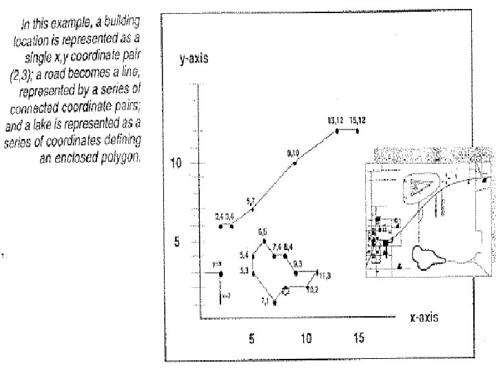
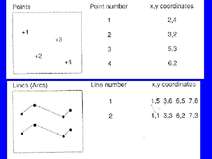
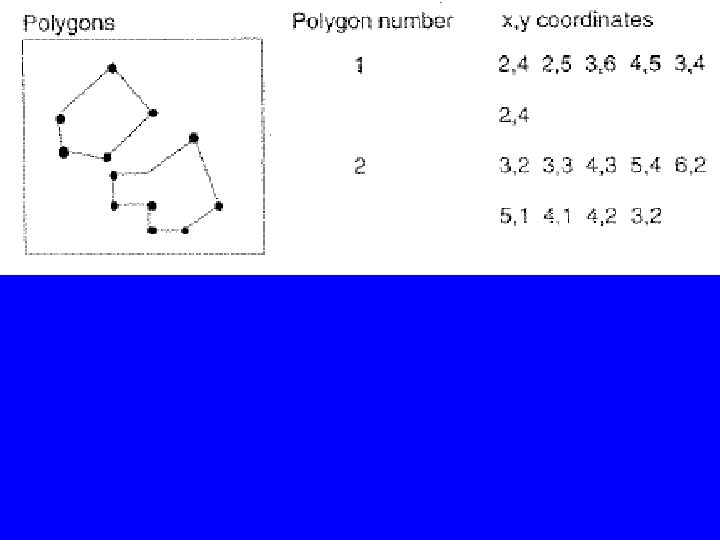
• In vector representation, each points is recorded as a single x, y location. Lines (arcs, or links) are recorded as a series of ordered x, y. Areas are recorded as a series of x, y coordinates defining arcs that enclose the area, first and last points are the same in this case. Areas can also be defined by the arcs around their boundaries, see figures. • This way, features are stored in terms of pairs of x, y coordinates instead of storing a graph. • Multiple features are represented by assigning an ID to each feature and list the pairs of coordinates against feature ID.

2 - Tabular (Descriptive) Data • Tabular data can include almost any data set, whether or not it contains geographic data. • Can be displayed: – on the view directly (by hyper linking? ); or – as descriptive (attribute) data that GIS links to map features. • Can be linked to map features through unique ID_s of the features • Often comes packaged with featured data. • May include description of locations by address or by coordinates for example.

Description of locations in tables can be displayed graphically. You can use a symbol to display the locations of bird nests or airport locations for example

Often stored in abbreviated way. A data dictionary describes the data not just full names. Very important to obtain a data dictionary when acquiring descriptive data

• An Arc. View map references the tabular data source it represents, but doesn't contain the tabular data itself. This means that tables are dynamic, because they reflect the current status of the source data they are based on. If the source data changes, a table based on this data will automatically reflect the change the next time you open the project containing this table. Data frames are also updated. • Formats supported by Arc. View: – Data from database servers such as Oracle, Ingres, Sybase, Informix, etc. – d. BASE III files – d. BASE IV files – INFO tables – Text files with fields separated by tabs or commas

3 - Image Data • Image data includes satellite images, aerial photographs, and other remotely sensed or scanned data • Image data is a form of raster data where each grid-cell, or pixel, has a certain value depending on how the image was captured and what it represents. For example, if the image is a remotely sensed satellite image, each pixel represents light energy reflected from a portion of the Earth's surface. If, however, the image is a scanned document, each pixel represents a brightness value associated with a particular point on the document. Arc. GIS refers to rasters as “surfaces” • Can be used as maps for analysis, background of a view or a map display, or as attributes linked to features.

Aerial photograph used as a map in the background Notice that locations of samples are displayed

Features can be drawn and displayed on top of images

• Arc. View -without extensions- supports images for display and attribute purposes only. They cannot be used for analysis since they are not feature based. In order to be able to create and analyze image data, “Spatial Analyst” must be added to Arc. View. • Arc. Map can handle raster data deeper. Images can be georefrenced and classified. • Scanned images used as attributes can also represent scanned text document such as permits.

A View or a data frame may Contain a single photograph

Images can be “hot linked” or “hyper-linked” to features.

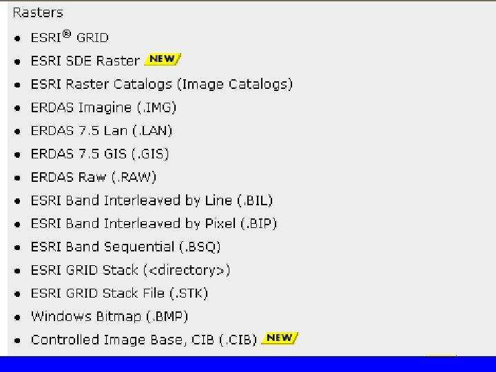
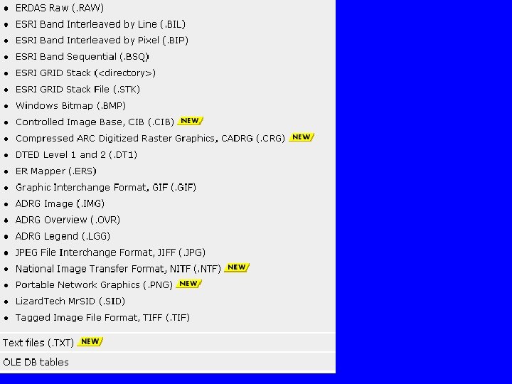
Arc. View supports the following image formats as themes: – ARC Digitized Raster Graphics (ADRG) (if Arc. View's ADRG Image Support extension is loaded) – BMP – BSQ, BIL and BIP – Compressed ARC Digitized Raster Graphics (CADRG) (if Arc. View's CADRG Image Support extension is loaded) – Controlled Image Base (CIB) (if Arc. View's CIB Image Support extension is loaded) – ERDAS – GRID

– IMAGINE (if Arc. View’s IMAGINE image extension is loaded) – IMPELL Bitmaps (Run-length compressed files) – Image catalogs – JPEG (if Arc. View’s JPEG image extension is loaded) – Mr. SID (if Arc. View’s Mr. SID image extension is loaded) – National Image Transfer Format (NITF) (if Arc. View's NITF Image Support extension is loaded) – Sun rasterfiles – TIFF/LZW compressed

Arc. View supports hot linking to the following image formats: (Notice that JPG is not supported in Version 3. 1 but supported in Arc. GIS) – GIF (Graphics Interchange Format) – Mac. Paint – Microsoft DIB (Device-Independent Bitmap) – Sun raster files – TIFF (Tag Image File Format) – TIFF/LZW compressed – X-Bitmap (generated by ‘bitmap' utility on X Windows) – XWD (X Windows Dump Format)

Acquiring Data • Certain considerations before acquiring data: (refer to attached sheet) – Area: consider an area that is not much larger and is not smaller than the area under study – Scale: the same feature is displayed differently at different scales. Roads can be lines or areas. Schools can be points or areas. Acquire data at a scale that fits your needs. – Time: some data change with time. If this is the case, make sure you obtain data at the time you want to consider. – Accuracy: location of roads within 40 ft is OK for traveling information but not for planning.

– Description: must obtain a data dictionary with the data, see attached data dictionary – Compatibility: the format of the data need to be supported by the software you are using. If not, it can be used only if you have a way of transforming the data into a format you can use.

• Sources of data: 1 - Governmental agencies provide them for a minimum charge. 2 - UW libraries have a huge collection of all sorts of data. Some of them are available on CD’s and some are available online. Check the sites: www. lib. washington. edu/maps/digdata. html wagda. lib. washington. edu {data for King County, Seattle, and WA state} wa-node. gis. washington. edu 3 - Vendors: all types of data at different scales are available for purchasing.

4 - The World Wide Web, became a very important source for free data check (www. esri. com), see attached sheet 5 - Users: users can create their own data by: 1 - digitizing from maps or images digitizing is the process of manually converting hard copy maps into digital format for use by a computer.

• Digitizers have their own internal coordinate systems, up to 0. 025 mm, which may be related to terrain coordinates by cross-registering

At least three points with known terrain coordinates. After registering the points, a cross hair or cursor is placed over the position to be recorded and a key is pressed.

• Digitizing includes the entry of thematic codes for object types and ID codes which link the object type to attribute data. For example, digitizing a building includes entry of thematic codes for buildings and ID number for a building. A new ID number is entered for the next building, and so on.

2 - drawing over maps or images 3 - from tables: features can be mapped based on their locations in tables, usually using symbols. Address geocoding helps translates addresses in tables into coordinates for display on maps. 4 - typing attribute tables.

Table of attributes

Storing Geographic Data • A digital map database consists of two types of information: spatial and descriptive data. • The computer stores a series of files that contain either type • The power of GIS lies in its ability to link the two types of data and maintain the spatial relationship between the map features (what is next to what? ) • Tabular data can be accessed from the map and can be used to create maps. For example, you can change the classification (colors) according to different attributes.

Tracts classified according to price

Tracts classified according to roof type

Tracts classified according to area

Representing Maps in the Computer • Features are represented by (points, lines or areas) or cells. • Features are referenced to ground locations through a two dimensional flat Cartesian system. • Spatial Data Models and Structures – Vector – Raster (surface in Arc. GIS) – Database (tables)

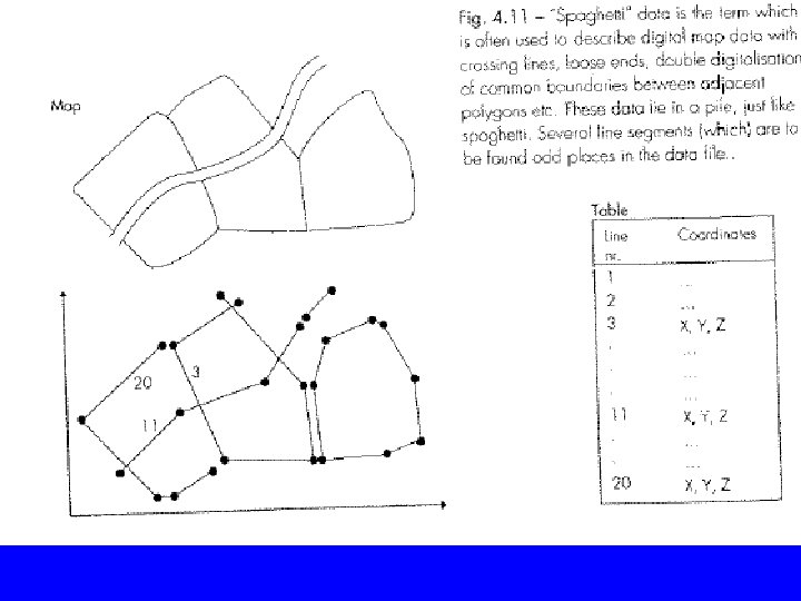
I- Vector Data Structures Vector data usually come in one of two data structures: A- Spaghetti • digital map data with crossing lines, loose ends, open shapes, double boundaries, etc. The data lie in a pile, just like spaghetti, see attached figure. • Takes large space to store and very hard to search through. • Not suitable for most GIS applications, no overlaying possible for example.

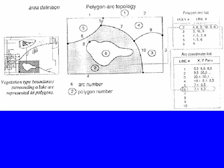
B- Topological data structure: Topology • Topology is a mathematical procedure for explicitly defining spatial relationships. • Example of spatial relationships: the route from the airport to a hotel. • Using topological relationships, data can be stored more efficiently and can be processed faster. • Three major topological relationships: – connectivity – area definition – contiguity

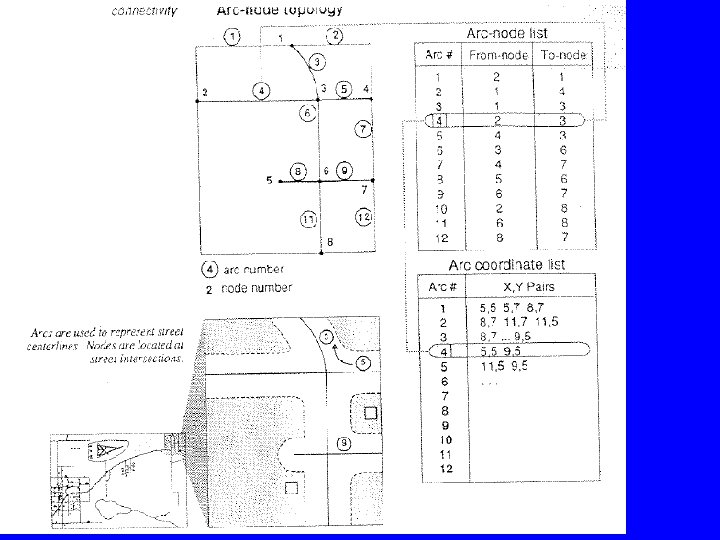
B. 1. Connectivity • Arcs connects to each others at nodes • Points along the arc are called vertices, points at the end of arcs are called nodes • Each arc has two nodes: a from-node and a to-node. • Arcs join only at nodes. That enables a GIS software to identify which arcs meet (connect) at a certain point (node). Consequently, the software can recognize that certain lines are connected, see figure • If two lines are connected, share the same node, then you can travel from one to the other?

B. 2. Area Definition • Arcs that connect to surround an area define a polygon • Areas can be defined by sets of x, y coordinates. • A more efficient way is to store the ID’s of the arcs defining the area. That allows for storing the arcs only once and insures that boundaries of adjacent polygons do not overlap, see figure. • In this case, we store a polygon-arc list and an arc -coordinates list.

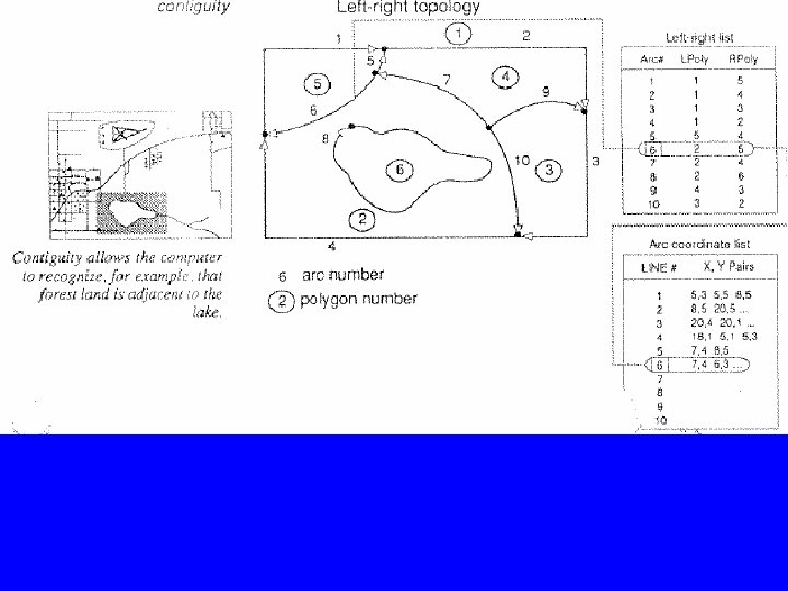
B. 3. Contiguity • Contiguity: arcs have directions, right and left arc; and each arc has a direction from the fromnode to the to-node. • A GIS software may store a left-right list which defines the polygons on the left and right sides of each arc, see figure. • Polygons sharing a common arc are adjacent. The left-right list describes the spatial arrangement of the areas, which one is to the left?

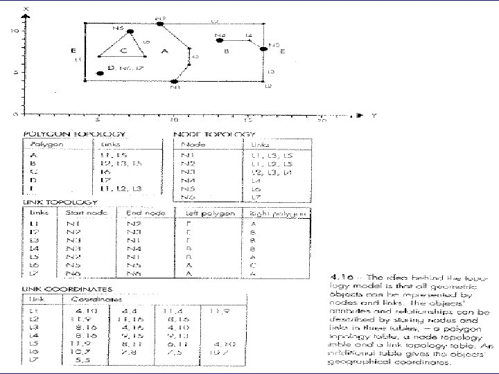
• Other topological data structures, see figure. • In summary, topological data structures define how points, lines, and polygons are related to each other on a map. • This relationship is obvious to the human eye, but needs to be explicitly defined to a computer. • Topological data structures may vary from a software to another, but they usually carry the same basic information.

Remarks about topological data structures • The connections and relationships between the objects are described. Their topology remains fixed as the geometry is stretched and bent. • Require that all lines be connected and all polygons be closed. No double boundaries. • Permit several spatial analysis such as overlaying, network analysis, contiguity analysis, and connectivity analysis • Less storage space, faster display and search • Take more time to construct and to update. • The prime choice in most GIS

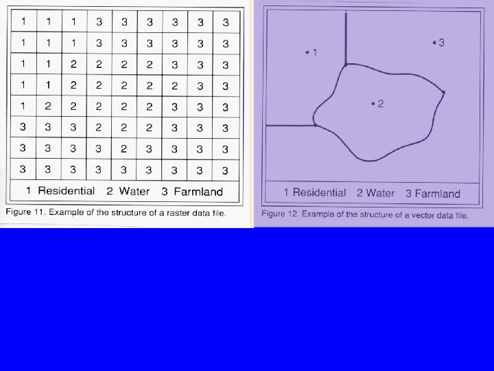
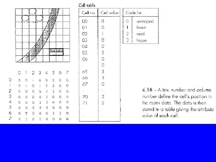
II- Raster (Grid) Data Model • Reality is represented in terms of uniform, regular cells (pixels: picture elements).

• Cells are usually rectangular or squares. • Geometric resolution of the model depends on the size of the cells. • The location of the cell is described in terms of its row and column. The numbering start at the top left cell being 00. • Cell locations in terms of rows and columns can easily be transformed into a Cartesian system by a two dimensional affine coordinate transformation (Row, Column) (X, Y)

Devils Tower, Wyoming 1: 24, 000 raster visualization of DTM

DTM of ground under canopy

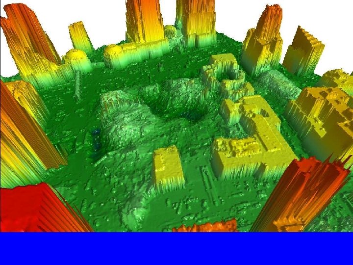
LIDAR images of the WTC by NOAA. Elevations are color coded http: //www. noaanews. noaa. gov/stories/s 781. htm

Dark Green -30 to 0 Green 0 to 98 Yellow 98 to 328 Magenta 328 to 492 Red 492 to 765 The 3 -D models have helped to locate original support structures, stairwells, elevator shafts, basements, etc.

• Cell values can represent many things: a gray level, a code for feature types, or any other attribute. • Figures 4. 17 and 4. 18

• A cell can be assigned a single value. That results in different themes as with the vector model. Figure 4. 19

• A single cell may cover parts of two or more objects or values. A classification scheme is followed to assign a value to the cell: average, largest, the one in the middle, etc. , figure 4 -18

• Spatial arrangements, topology in vector models, may be achieved by a search of the neighboring cells, takes more time. • Storing raster data – can be stored in the form of a table: location and value. – many compression algorithms are available. Run-length encoding simply stores the number of consecutive similar cells: 4 x 2 w 3 r 1 x 3 x, and so on. Figure 4. 22

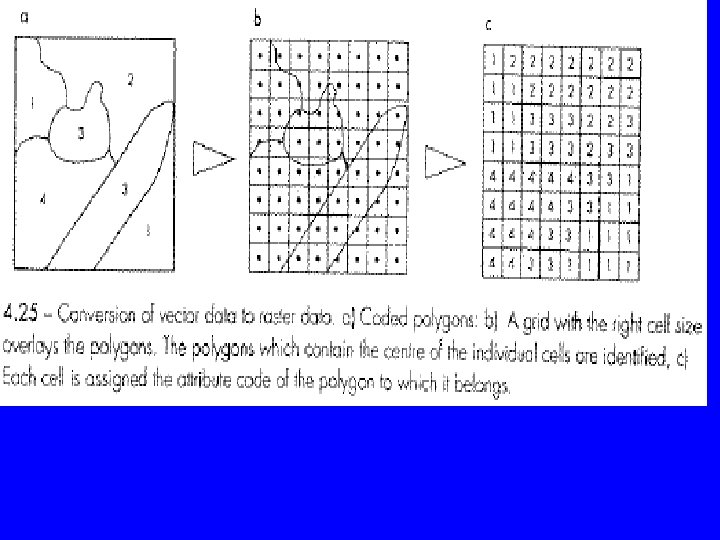
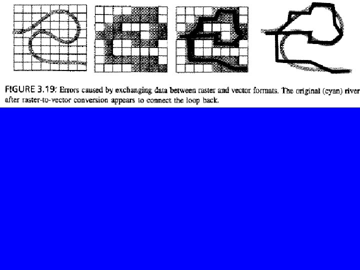
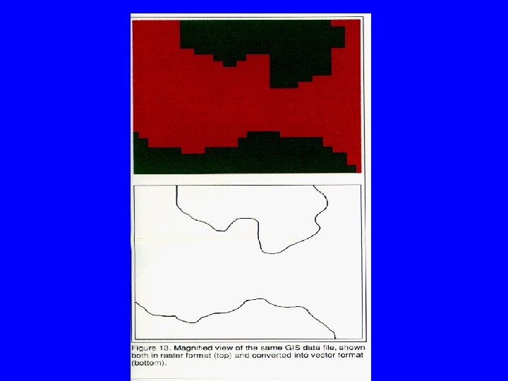
• Vectorisation and rasterisation – transforming raster into vector or vector into raster format respectively. – can be done automatically within the software – part of the data is lost in the transformation process, why? Figures 4 -24, and 4 -25

Vector VS Raster Models • Raster models are superior in handling phenomena that are related to areas and points while vector models handle line-related phenomena better. • Overlaying in particular is faster with raster models • Raster models are easier to produce from hard copies by scanning, vector models require digitization which is time consuming. • Raster models require larger storage space and more powerful computing system. • Raster models are more suitable for many presentation purposes, DEMs for example are lot easier to visualize in a raster format.

Overlay in vector representation

Overlay in raster representation

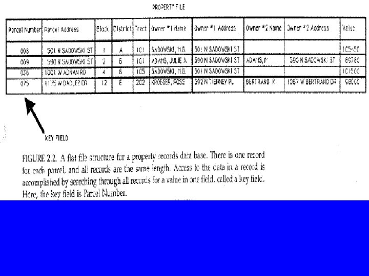
III- Database Structures • A data base is simply a collection of multiple files. • A GIS is, first and foremost, an information system • There is a need for an efficient data management system to facilitate the integration and cross referencing between different types of data. 1 - Flat Files – All the information about a feature are stored in a single record. All rows have the same number of columns which may result in empty cells. – Search is done through a key field (attribute) – A structure that results in a slow system that requires huge storage. Fig 2. 3 of Huxhold

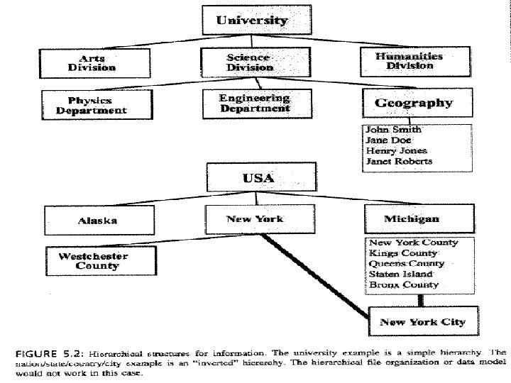
2 - Hierarchical Files – More than one type of record in the data base (many tables) – One record can be a parent of one or more records in another table through pointers. – One way relationship which reduces repetition of information. – Each record can have one parent only. – Very useful in one-to-many situations, Arc. GIS will append the first maching record only in that case. – Allows limited linking process, pointers are pre-set in the design.

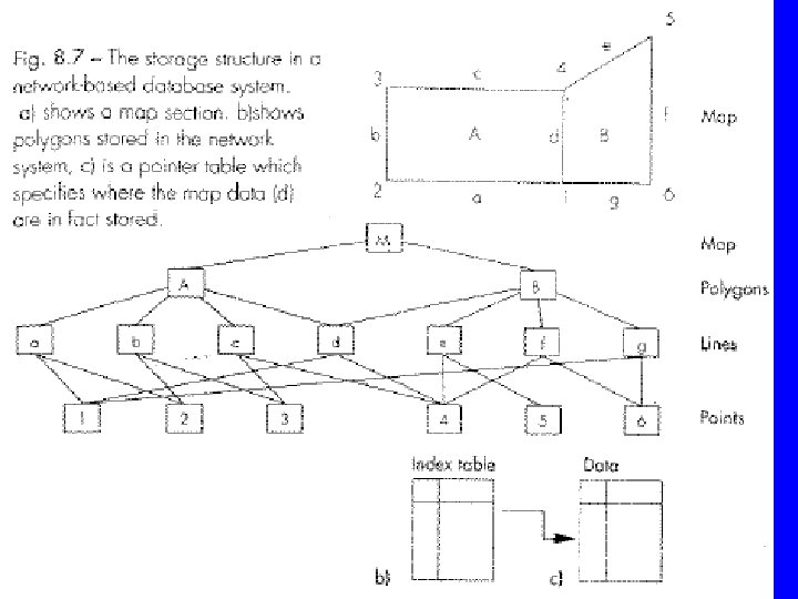
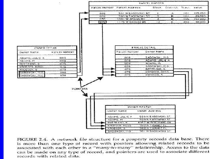
3 - Networks – Records are not necessarily unique. One feature having more than one value of a certain attribute may show up twice. For example, owners of many parcels. – Pointers allow many-to-many relationship, one record may have more than one parent. Still one way relationship. – Pointers may become very complicated and may occupy larger space than the data itself. Figure 8 -7 Tor.

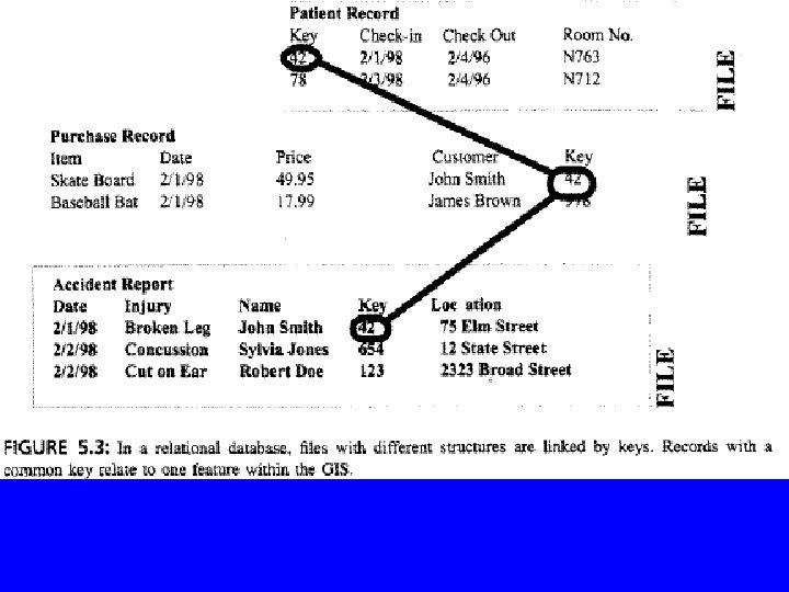
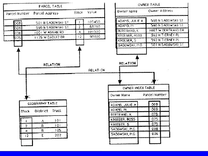
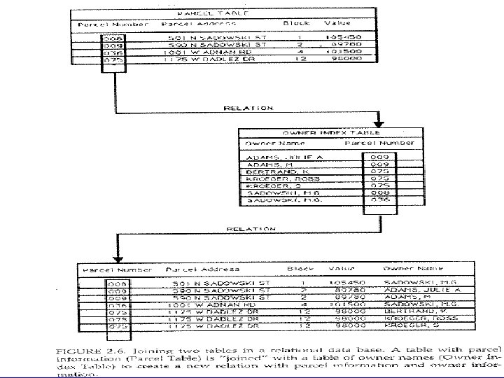
4 - Relational databases – Allows related records from different files to be associated with each other through a common attribute without pointers between the records (the rows) – They contain a group of flat files that can be related in any direction. – Tables can be joined to form new tables by choosing any common field (column) – Fast and flexible structure. Does not require large storage for the links. – Figures 2. 5 and 2. 6 of Huxhold. – The most common data base structure in modern GIS software. Definition: Relational Data Base A data model based on set theory. Each set has elements that can be uniquely defined by a primary key. A table (relation) stores all records for a set. Each record in a table has the same columns for attribute values. Relationships between tables are constructed by storing the key to a record in the other table

Referencing Spatial Data

• GIS data must be in the same system, based on the same ellipsoid, and the same projection. • We will look into: – Vertical Reference in the US “elevations” – Horizontal Reference • Global Systems: Geodetic “ geographic” and UTM • Local system: State Plane Coordinate System

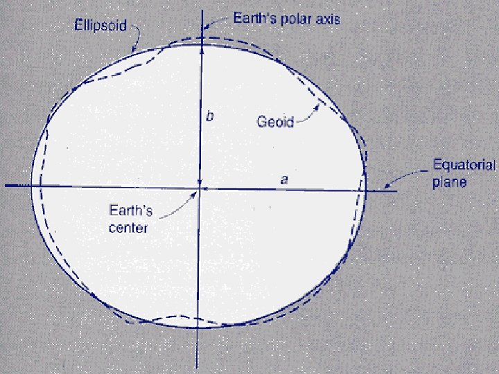
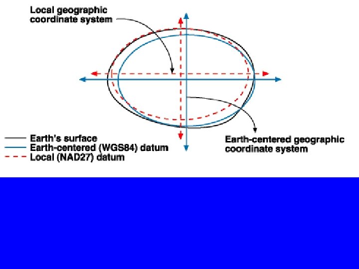
Shape of the Earth • Geoid and Ellipsoid, what for? • A geoid is a surface of equal gravity from which elevations are measured, cannot be mathematically defined easily. • An ellipsoid is an approximation of a geoid to produce a mathematically defend surface, based on which horizontal coordinates can be defined.

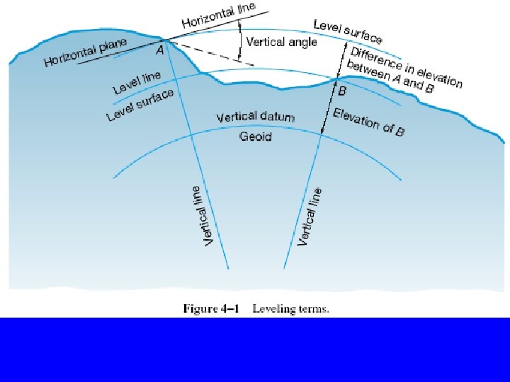
Vertical Reference “Elevations” {Based on Geoids}

• Vertical Datum: A level surface to which elevations are referred, for example: MSL. A geoid “surface of equal gravity” that contains large water bodies • Elevation: the vertical distance from a vertical datum to a point or an object.

North American Vertical Datum • Started in 1850’s, first phase completed in 1929 • Thousands of Points across the US and Canada were related to MSL and adjusted, the newly defined MSL defined a new datum called: National Geodetic Vertical Datum of 1929, or (NGVD 29) • Due to the earth’s crust shifting and changes in MSL, new adjustment was done and more points were added (total of 1. 3 million) which resulted in NAVD 88 • Shifts are larger in the west: 1. 5 m in the Rocky mountain area • MUST MENTION WHICH DATUM

Horizontal Reference {Based on Ellipsoids}

• The locations of map features are referenced to actual locations of the objects they represent in the real world. • The positions of objects on the earth’s spherical (ellipsoidal) surface are usually given in degrees of latitude and longitude, also known as geographic or geodetic coordinates. • On a flat map, the locations of features are measured in a two dimensional planner coordinate system. Examples are state plane coordinate system or UTM.

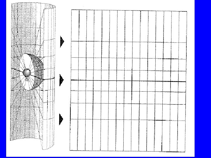
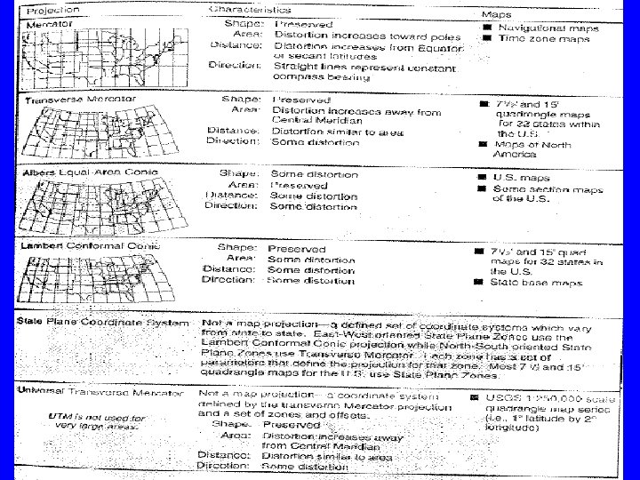
Map Projections • Because the earth is round and maps are flat, getting information from the curved to the flat surface requires a mathematical operation called map projection. • We mathematically project data from the surface of a certain ellipsoid to a flat surface we call a map. • Map projection is a transformation process, it transforms and into x and y coordinates. • Flattening the earth result in distortions in: distance, area. shape, and directions. All maps are distorted in some of these spatial properties.

• Some map projections minimize distortions in one property on the expense of another, while others balance the overall distortions. • All the data in a GIS database must be in the same map projection. Better to store locations in unprojected coordinates (decimal degrees)

Longitudes and latitudes are considered as a simple two dimensional coordinate system

Conformal: scale is equal on all directions, parallels and meridians drawn at right angles. Small areas and angles with small sides are correct.

Equal-Area: areas are equal to those on ground. Maps cannot be Equal-Area and conformal

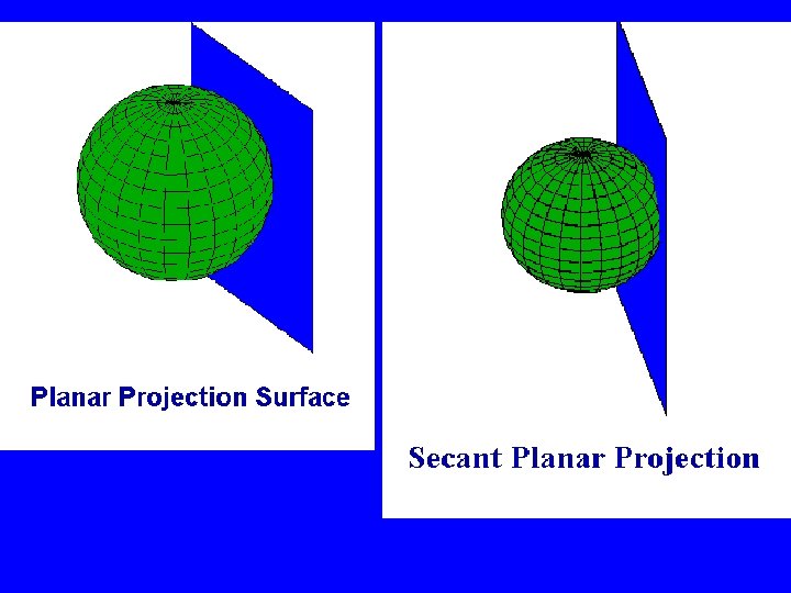
Distances and directions along the center are correct. This “Polar” map was projected onto a plan tangent at the north pole

Which ellipsoid? • Define ellipsoid parameters (equations not required): • semi-major axes (a), semi-minor axes (b) e= = first eccentricity • N = normal length = • • Two main ellipsoids in North America: Clarke ellipsoid of 1866, on which NAD 27 is based • Geodetic Reference System of 1980 (GRS 80): on which NAD 83 is based. • For lines up to 50 km, a sphere of equal volume can be used •

Horizontal Reference Coordinate Systems {Based on Ellipsoids} Global Systems 1 - Geodetic “geographic” 2 - UTM

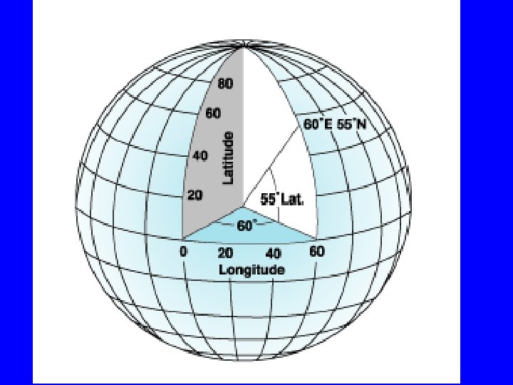
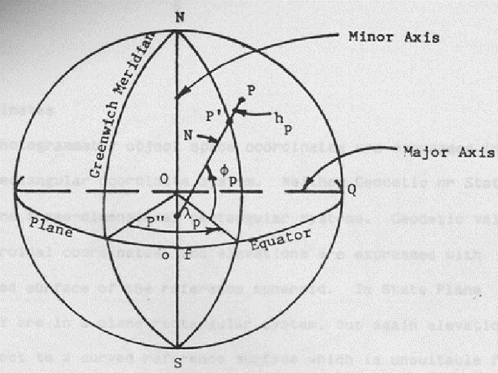
1 - Geodetic “geographic” Coordinate System • A global System that is defined anywhere on earth, no distortions. • Definitions : – Geodetic latitude (f): the angle in the meridian plane of the point between the equator and the normal to the ellipsoid through that point. – Geodetic longitude (l): the angle along the equator between the Greenwich and the point meridians – Height above the ellipsoid (h)

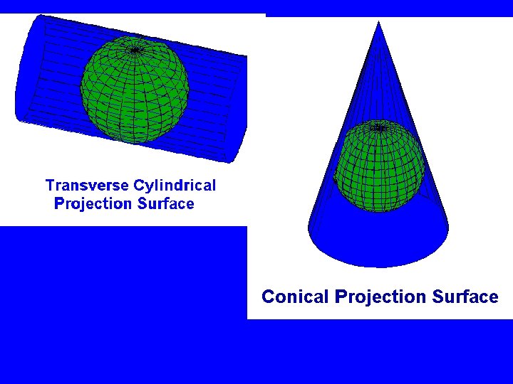
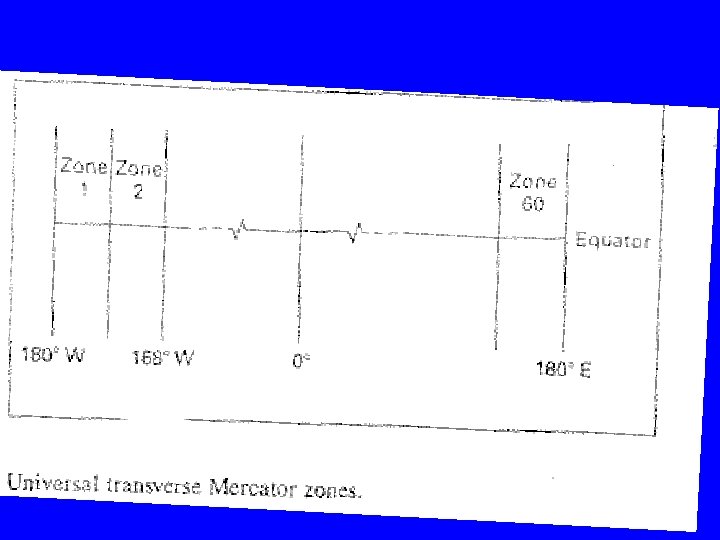
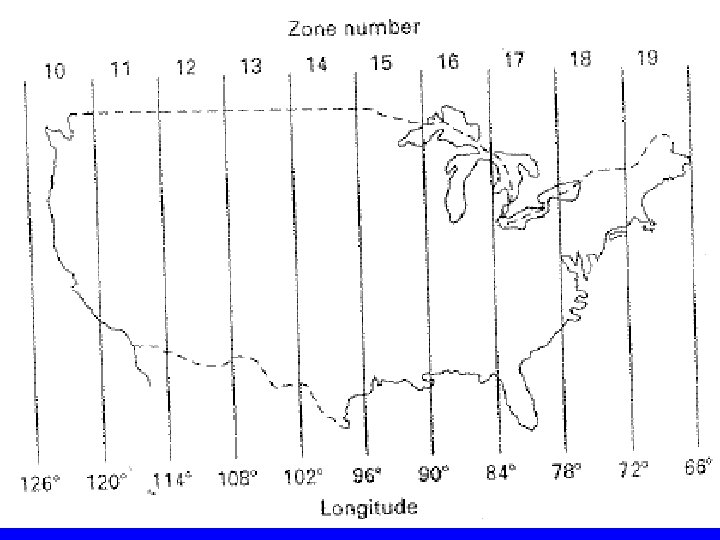
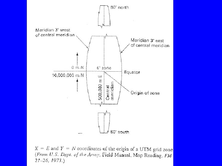
2 - Universal Transverse Mercator (UTM) • Preserves shapes. • Based on the transverse mercator projection • In zones that are 6 degrees wide, 3 in military applications • The unit of measure is meter • Zones are numbered beginning with 1 for the zone between 180 W and 174 W meridians. Zone numbers increase to a maximum of 60. • The latitude for the system varies from 80 N to 80 S.

• The origin of longitude is at the central meridian • False easting is 500, 000 m at central meridian. • The origin of latitude is at the equator • False northing is 0 for the northern hemisphere and is 10, 000 m for the southern hemisphere. • A global system used in USGS 1: 250, 000 scale quadrangle map series.

Coordinate Systems Local US Systems State Plane Coordinate Systems

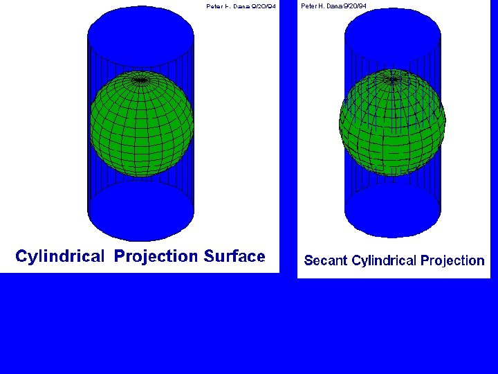
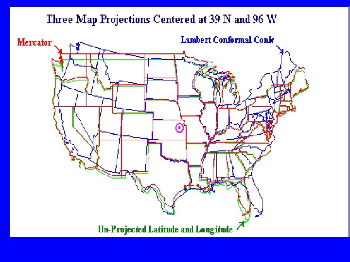
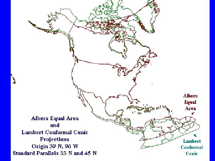
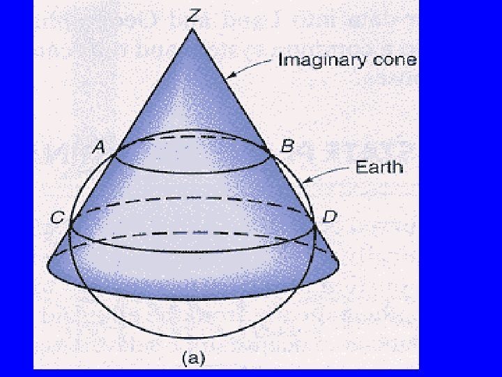
“LOCAL” State Plane Coordinate Systems • Plane rectangular systems, why use them? • How to construct them: Project the earth’s surface onto a developable surface. • Two major projections: Lambert Conformal Conic, and Transverse Mercator.

Secants, Scales, and Distortions • Scale is exact along the secants, smaller than true in between. • Distortions are larger away from the secants

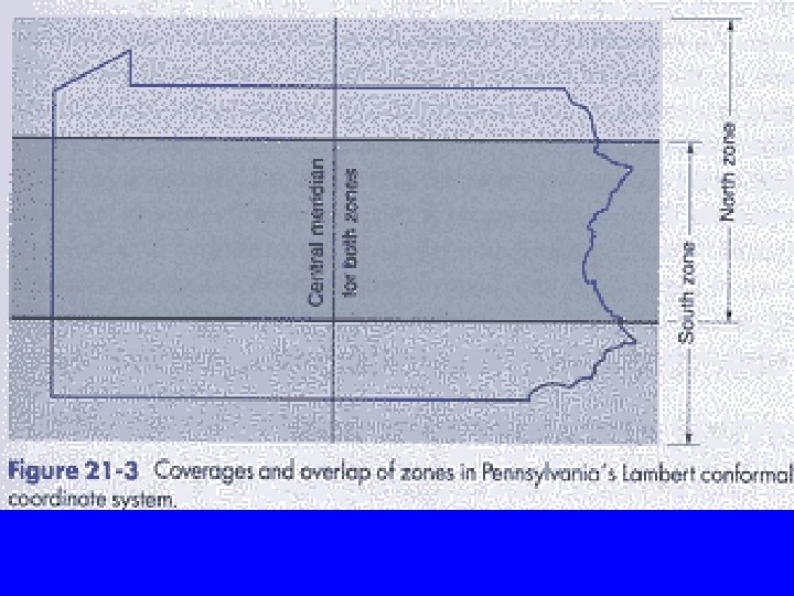
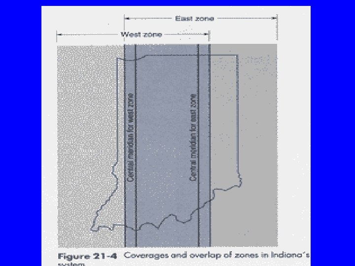
How They Selected Projections? • States extending East-west: Lambert Conical • States extending North-South: Mercator Cylindrical. • A single surface will provide a single zone. Maximum zone width is 158 miles to limit distortions to 1: 10, 000. States longer than 158 mi, use more than one zone (projection).

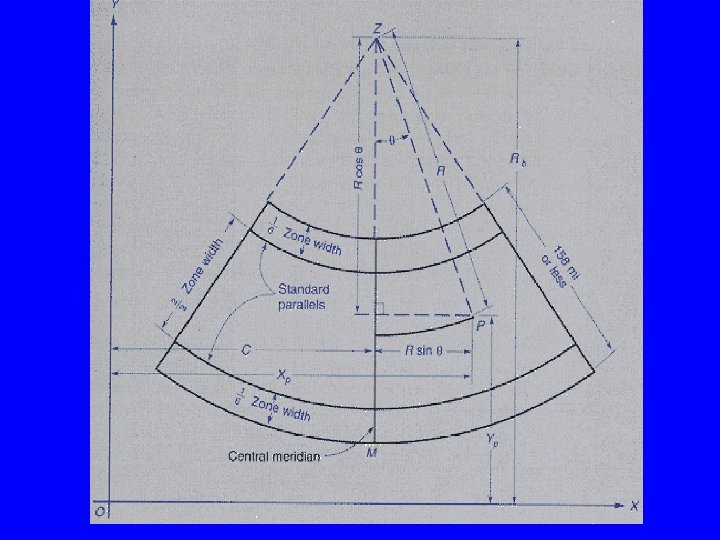
Standard Parallels & Central Meridians • Standard Parallels: the secants, no distortion along them. At 1/6 of zone width from zone edges • Central Meridians: a meridian at the middle of the zone, defines the direction of the Y axis. • The Y axis points to the grid north, which is the geodetic north only at the central meridian

Geodetic and SPCS • Control points in SPCS are initially computed from Geodetic coordinates. • If NAD 27 is used the result is SPCS 27. If NAD 83 is used, the result is SPCS 83.