The Nature of Geographic Data The Paper Map

The Nature of Geographic Data

The Paper Map • A long and rich history • Has a scale or representative fraction – The ratio of distance on the map to distance on the ground • Is a major source of data for GIS – Obtained by digitizing or scanning the map and registering it to the Earth’s surface • Digital representations are much more powerful than their paper equivalents

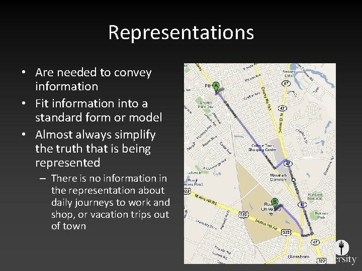
Representations • Are needed to convey information • Fit information into a standard form or model • Almost always simplify the truth that is being represented – There is no information in the representation about daily journeys to work and shop, or vacation trips out of town

Digital Representation • Uses only two symbols, 0 and 1, to represent information – N symbols (bits) 2 N distinct values • Many standards allow various types of information to be expressed in digital form – MP 3 for music – JPEG for images – ASCII for text • GIS relies on standards for geographic data

Why Digital? • Economies of scale – One type of information technology for all types of information • Simplicity – 0, 1 on, off • Reliability – Systems can be designed to correct errors • Easily copied and transmitted – Perfect copies – At close to the speed of light

Accuracy of Representations • Representations can rarely be perfect – Details can be irrelevant, or too expensive and voluminous to record • It’s important to know what is missing in a representation – Representations can leave us uncertain about the real world

The Fundamental Problem • Geographic information links a place, and often a time, with some property of that place (and time) – “The temperature at 34 N, 120 W at noon local time on 12/2/99 was 18 Celsius” • The potential number of properties is vast – In GIS we term them attributes – Attributes can be physical, social, economic, demographic, environmental, etc.

Types of Attributes • Nominal, e. g. land cover class – Distinction (“a” is/is not “b”) • Ordinal, e. g. a ranking – Significance (“a” is X-er than “b”) • Interval, e. g. Celsius temperature – Relative magnitude (“a” is N units X-er than “b”) • interpolable • Ratio, e. g. Kelvin temperature – Absolute magnitude (“a” is N times X-er than “b”) • scalable

Cyclic Attributes • Do not behave as other attributes – What is the average of two compass bearings, e. g. 350 and 10? • Occur commonly in GIS – Wind direction – Slope aspect – Flow direction • Special methods are needed to handle and analyze

The Fundamental Problem • The number of places and times is also vast – Potentially infinite • The more closely we look at the world, the more detail it reveals – Potentially ad infinitum – The geographic world is infinitely complex • Humans have found ingenious ways of dealing with this problem – Many methods are used in GIS to create representations or data models

Types of Spatial Data • Discrete: definitive; with concrete, observable, boundaries • Continuous: no easily discernable boundaries, “fuzziness” depends on scale

Types of Spatial Data • Continuous spatial data: geostatistics – Samples may be taken at intervals, but the spatial process is continuous – e. g. soil quality • Discrete data – Irregular: zonal data, regions, states, districts, postcodes, zipcodes – Regular lattice data: constructed grid, ‘raster’ representation

Discrete Objects and Fields • Two ways of conceptualizing geographic variation – The most fundamental distinction in geographic representation • Discrete objects – The world as a table-top – Objects with well-defined boundaries

Discrete Objects • • Points, lines, and areas Countable Persistent through time, perhaps mobile Biological organisms – Animals, trees • Human-made objects – Vehicles, houses, fire hydrants

Fields • Properties that vary continuously over space – Value is a function of location – Property can be of any attribute type, including direction • Elevation as the archetype – A single value at every point on the Earth’s surface – The source of metaphor and language • Any field can have slope, gradient, peaks, pits

Examples of Fields • Soil properties, e. g. p. H, soil moisture • Population density – But at fine enough scale the concept breaks down • • Name of county or state or nation Atmospheric temperature, pressure Pollution level Groundwater quality information

Difficult Cases • Lakes and other natural phenomena – Often conceived as objects, but difficult to define or count precisely – “When is a heap of sand no longer a heap? ” • Weather forecasting – Forecasts originate in models of fields, but are presented in terms of discrete objects • Highs, lows, fronts

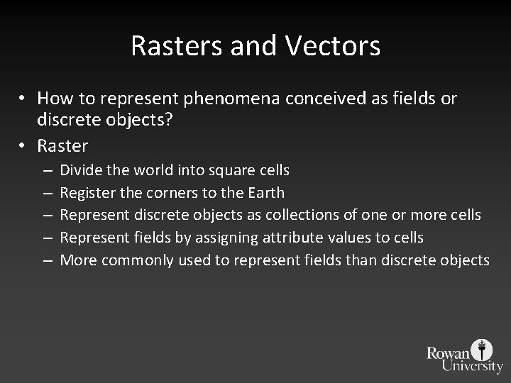
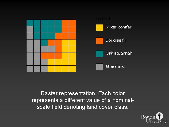
Rasters and Vectors • How to represent phenomena conceived as fields or discrete objects? • Raster – – – Divide the world into square cells Register the corners to the Earth Represent discrete objects as collections of one or more cells Represent fields by assigning attribute values to cells More commonly used to represent fields than discrete objects

Legend Mixed conifer Douglas fir Oak savannah Grassland Raster representation. Each color represents a different value of a nominalscale field denoting land cover class.

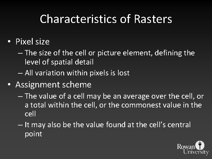
Characteristics of Rasters • Pixel size – The size of the cell or picture element, defining the level of spatial detail – All variation within pixels is lost • Assignment scheme – The value of a cell may be an average over the cell, or a total within the cell, or the commonest value in the cell – It may also be the value found at the cell’s central point

Vector Data • Used to represent points, lines, and areas • All are represented using coordinates – One per point – Areas as polygons • Straight lines between points, connecting back to the start • Point locations recorded as coordinates • May have “holes” and “islands” – Lines as polylines • Straight lines between points

Raster vs Vector • Volume of data – Raster becomes more voluminous as cell size decreases • Source of data – Remote sensing, elevation data come in raster form – Vector favored for administrative or discrete data • Software – Some GIS better suited to raster, some to vector

Generalization • GIS data may preserve data beyond what you need or want • Arc. GIS can differentiate between incredibly small values – State Plane (feet) default is 0. 003937 inches • Software may have difficulties displaying overly detailed data at smaller scales

Spatial Autocorrelation • First law of geography: “everything is related to everything else, but near things are more related than distant things” – Waldo Tobler • Many new geographers would say “I don’t understand spatial autocorrelation” Actually, they don’t understand the mechanics, they do understand the concept.

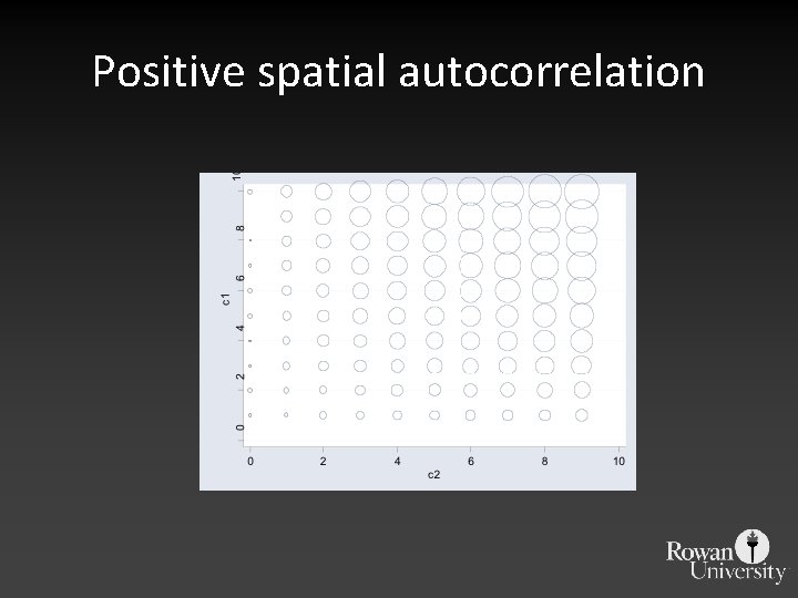
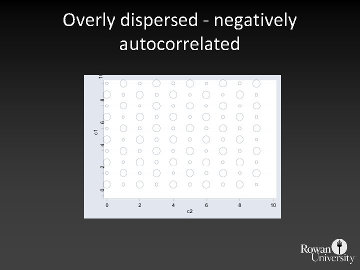
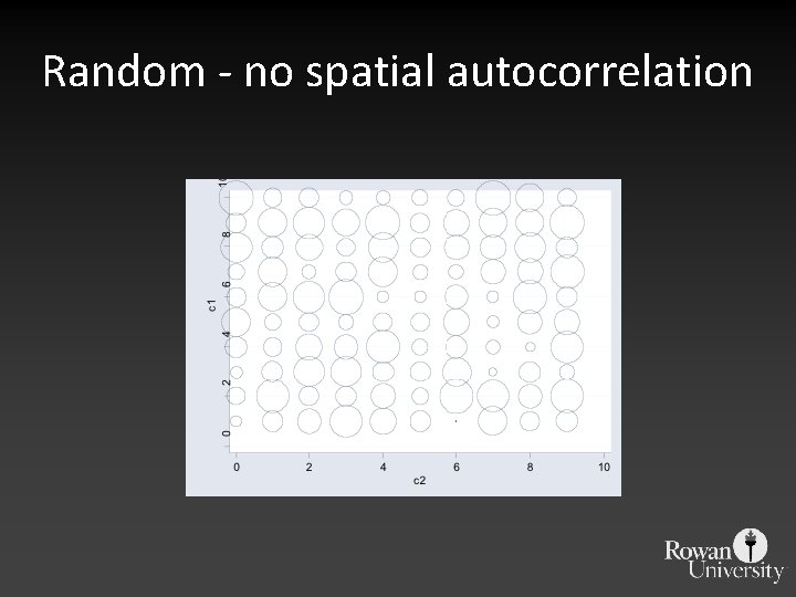
Spatial Autocorrelation • Spatial Autocorrelation – correlation of a variable with itself through space. – If there is any systematic pattern in the spatial distribution of a variable, it is said to be spatially autocorrelated – If nearby or neighboring areas are more alike, this is positive spatial autocorrelation – Negative autocorrelation describes patterns in which neighboring areas are unlike – Random patterns exhibit no spatial autocorrelation

Positive spatial autocorrelation

Overly dispersed - negatively autocorrelated

Random - no spatial autocorrelation

Importance of Spatial Autocorrelation • Most statistics are based on the assumption that the values of observations in each sample are independent of one another • Positive spatial autocorrelation may violate this, if the samples were taken from nearby areas • Goals of spatial autocorrelation – Measure the strength of spatial autocorrelation in a map – test the assumption of independence or randomness

Why does spatial auto correlation occur? • Reaction functions? • Spillovers, externalities? • Unobserved similarities between places? • Diffusion? (disease spread) • Common activity in neighboring areas? (crime) • Common policy across neighboring areas? (zoning)

Sampling • The sampling density determines the resolution of the data • Samples taken at 1 km intervals will miss variation smaller than 1 km • Standard approaches to sampling: – Random – Systematic – Stratified

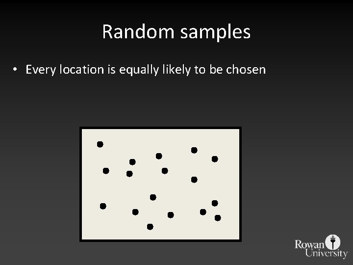
Random samples • Every location is equally likely to be chosen

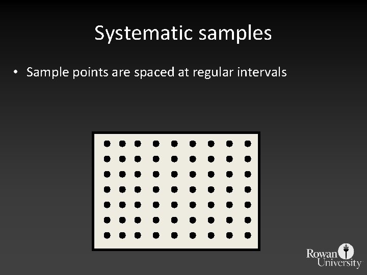
Systematic samples • Sample points are spaced at regular intervals

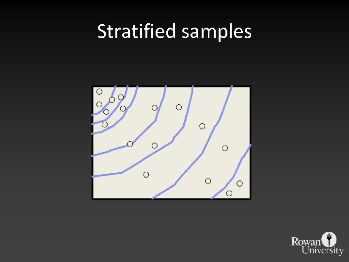
Stratified samples • Requires knowledge about distinct, spatially defined sub -populations (spatial subsets such as ecological zones) • More sample points are chosen in areas where higher variability is expected

Stratified samples

Using (Geospatial) Statistics • As always, error propagates and grows through subsequent analyses • Correlation does not mean causation • Sampling method may introduce bias • Models and measurements must be appropriate for your dataset • With GIS data, model must be geo-aware

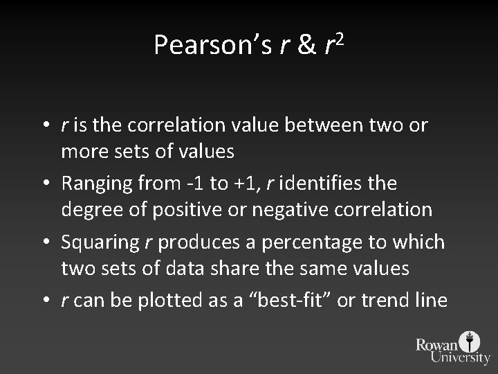
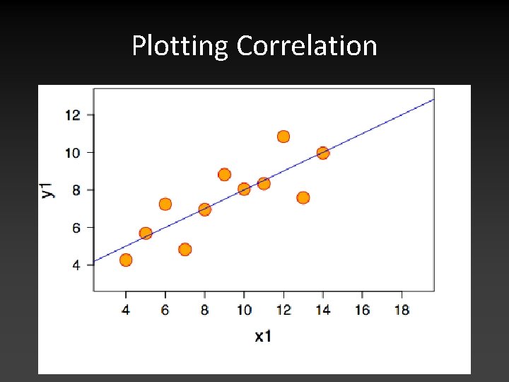
Pearson’s r & r 2 • r is the correlation value between two or more sets of values • Ranging from -1 to +1, r identifies the degree of positive or negative correlation • Squaring r produces a percentage to which two sets of data share the same values • r can be plotted as a “best-fit” or trend line

Plotting Correlation

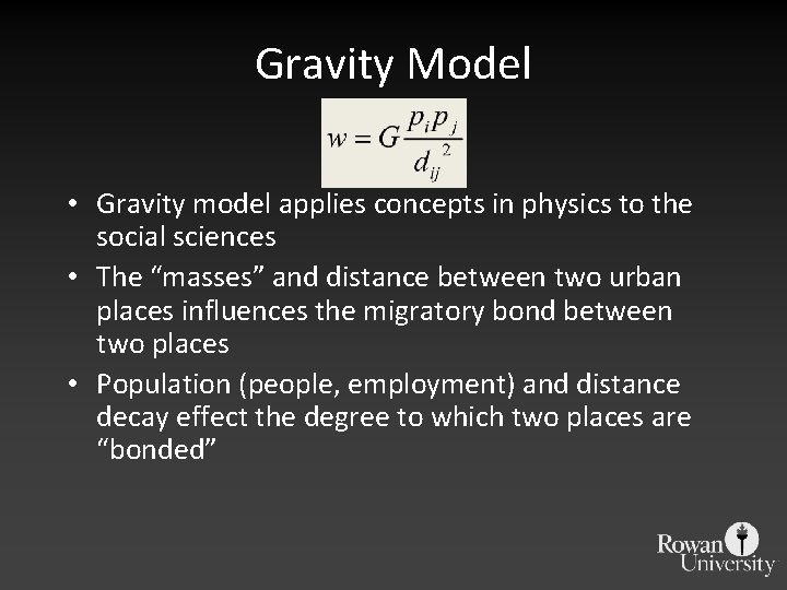
Gravity Model • Gravity model applies concepts in physics to the social sciences • The “masses” and distance between two urban places influences the migratory bond between two places • Population (people, employment) and distance decay effect the degree to which two places are “bonded”

Self-similarity and fractals

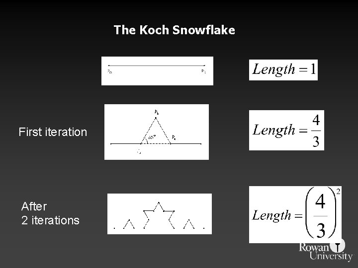
The Koch Snowflake First iteration After 2 iterations

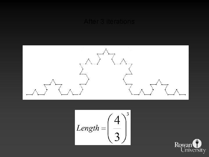
After 3 iterations

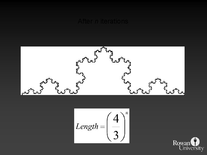
After n iterations

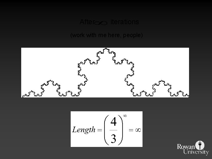
After iterations (work with me here, people)

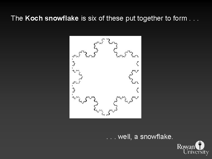
The Koch snowflake is six of these put together to form. . . well, a snowflake.

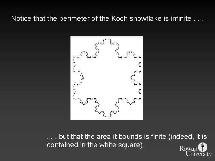
Notice that the perimeter of the Koch snowflake is infinite. . . but that the area it bounds is finite (indeed, it is contained in the white square).

Importance of Fractals • The precision at which you measure linear features influences the total length • What measurement is “right”? • Self-similarity of features – A craggy shoreline will have a similar pattern at a small and large scale – An agglomeration of urban neighborhoods into a city mirrors the pattern of cities creating a region

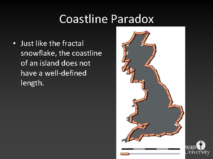
Coastline Paradox • Just like the fractal snowflake, the coastline of an island does not have a well-defined length.