For Monday Finish reading chapter 18 Homework Chapter

For Monday • Finish reading chapter 18 • Homework: – Chapter 18, exercises 1 and 2

Program 3 • Any questions?

Training Experience Issues • Direct or Indirect Experience – Direct: Chess boards labeled with correct move extracted from record of expert play. – Indirect: Potentially arbitrary sequences of moves and final games results. • Credit/Blame assignment: – How do we assign blame to individual choices or moves when given only indirect feedback?

More on Training Experience • Source of training data: – “Random” examples outside of learner’s control (negative examples available? ) – Selected examples chosen by a benevolent teacher (near misses available? ) – Ability to query oracle about correct classifications. – Ability to design and run experiments to collect one's own data. • Distribution of training data: – Generally assume training data is representative of the examples to be judged on when tested for final performance.

Concept Learning • The most studied task in machine learning is inferring a function that classifies examples represented in some language as members or non members of a concept from pre classified training examples. • This is called concept learning, or classification.

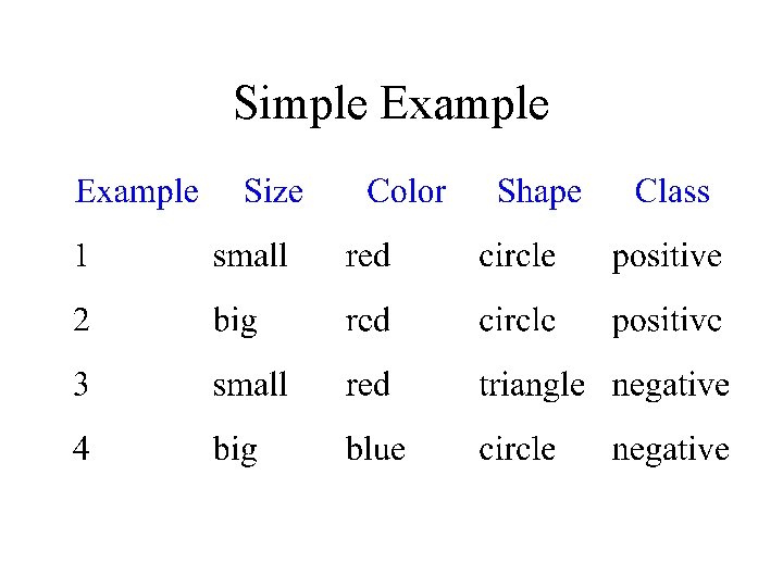
Simple Example

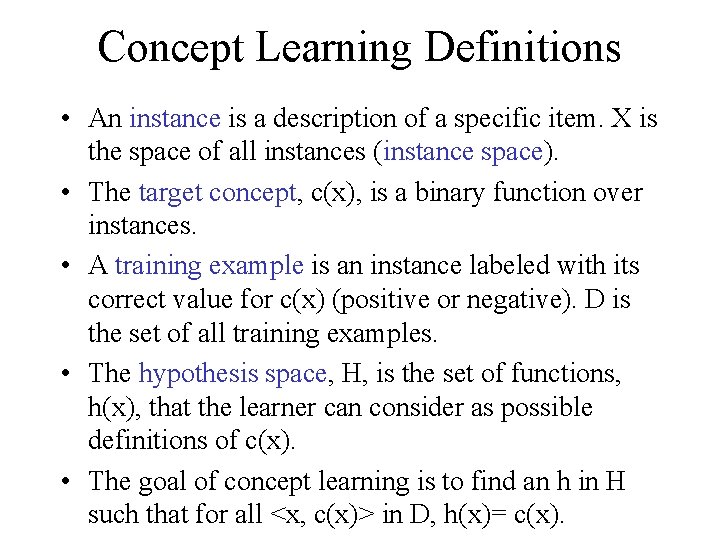
Concept Learning Definitions • An instance is a description of a specific item. X is the space of all instances (instance space). • The target concept, c(x), is a binary function over instances. • A training example is an instance labeled with its correct value for c(x) (positive or negative). D is the set of all training examples. • The hypothesis space, H, is the set of functions, h(x), that the learner can consider as possible definitions of c(x). • The goal of concept learning is to find an h in H such that for all <x, c(x)> in D, h(x)= c(x).

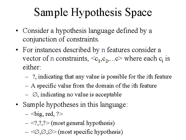
Sample Hypothesis Space • Consider a hypothesis language defined by a conjunction of constraints. • For instances described by n features consider a vector of n constraints, <c 1, c 2, . . . c> where each ci is either: – ? , indicating that any value is possible for the ith feature – A specific value from the domain of the ith feature – Æ, indicating no value is acceptable • Sample hypotheses in this language: – <big, red, ? > – <? , ? > (most general hypothesis) – <Æ, Æ, Æ> (most specific hypothesis)

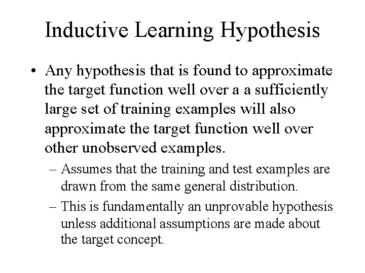
Inductive Learning Hypothesis • Any hypothesis that is found to approximate the target function well over a a sufficiently large set of training examples will also approximate the target function well over other unobserved examples. – Assumes that the training and test examples are drawn from the same general distribution. – This is fundamentally an unprovable hypothesis unless additional assumptions are made about the target concept.

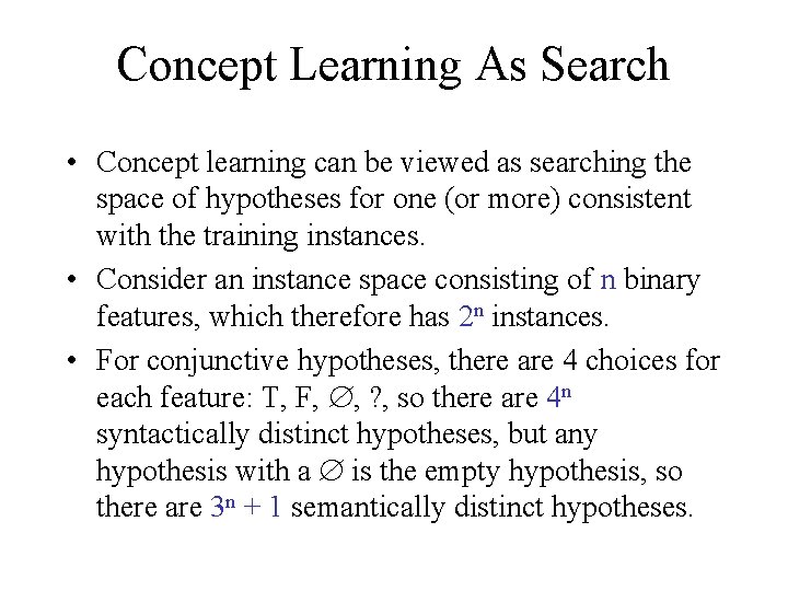
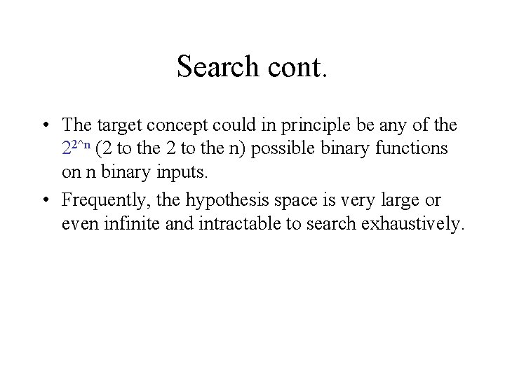
Concept Learning As Search • Concept learning can be viewed as searching the space of hypotheses for one (or more) consistent with the training instances. • Consider an instance space consisting of n binary features, which therefore has 2 n instances. • For conjunctive hypotheses, there are 4 choices for each feature: T, F, Æ, ? , so there are 4 n syntactically distinct hypotheses, but any hypothesis with a Æ is the empty hypothesis, so there are 3 n + 1 semantically distinct hypotheses.

Search cont. • The target concept could in principle be any of the 22^n (2 to the n) possible binary functions on n binary inputs. • Frequently, the hypothesis space is very large or even infinite and intractable to search exhaustively.

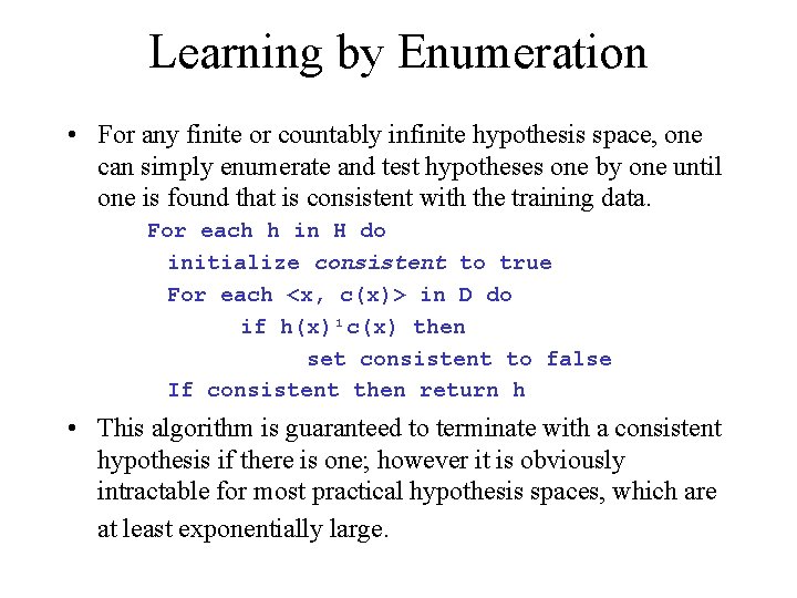
Learning by Enumeration • For any finite or countably infinite hypothesis space, one can simply enumerate and test hypotheses one by one until one is found that is consistent with the training data. For each h in H do initialize consistent to true For each <x, c(x)> in D do if h(x)¹c(x) then set consistent to false If consistent then return h • This algorithm is guaranteed to terminate with a consistent hypothesis if there is one; however it is obviously intractable for most practical hypothesis spaces, which are at least exponentially large.

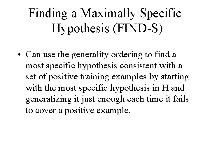
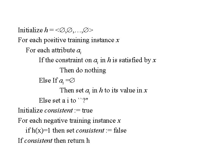
Finding a Maximally Specific Hypothesis (FIND S) • Can use the generality ordering to find a most specific hypothesis consistent with a set of positive training examples by starting with the most specific hypothesis in H and generalizing it just enough each time it fails to cover a positive example.

Initialize h = <Æ, Æ, …, Æ> For each positive training instance x For each attribute ai If the constraint on ai in h is satisfied by x Then do nothing Else If ai =Æ Then set ai in h to its value in x Else set a i to ``? '' Initialize consistent : = true For each negative training instance x if h(x)=1 then set consistent : = false If consistent then return h

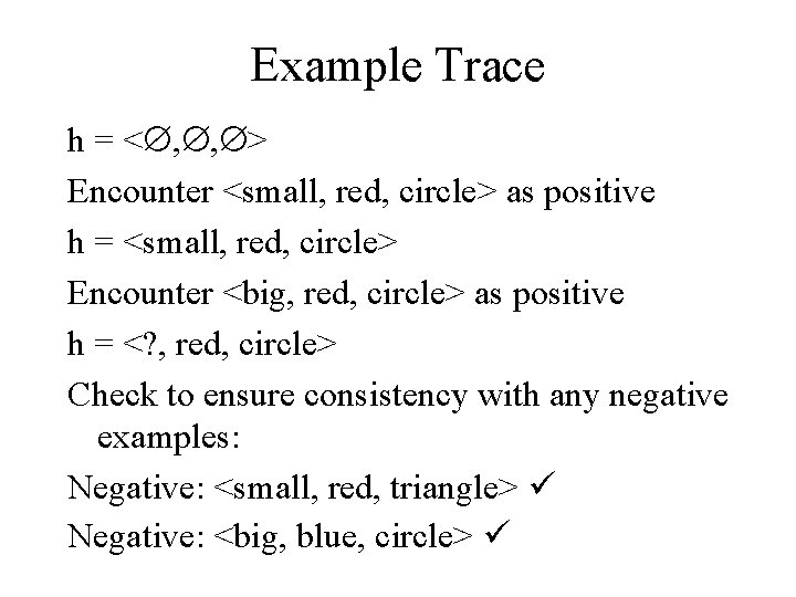
Example Trace h = <Æ, Æ, Æ> Encounter <small, red, circle> as positive h = <small, red, circle> Encounter <big, red, circle> as positive h = <? , red, circle> Check to ensure consistency with any negative examples: Negative: <small, red, triangle> Negative: <big, blue, circle>

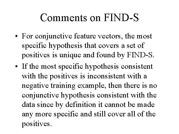
Comments on FIND S • For conjunctive feature vectors, the most specific hypothesis that covers a set of positives is unique and found by FIND S. • If the most specific hypothesis consistent with the positives is inconsistent with a negative training example, then there is no conjunctive hypothesis consistent with the data since by definition it cannot be made any more specific and still cover all of the positives.

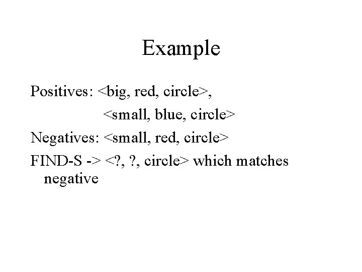
Example Positives: <big, red, circle>, <small, blue, circle> Negatives: <small, red, circle> FIND S > <? , circle> which matches negative

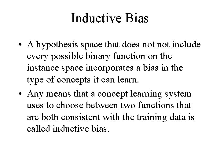
Inductive Bias • A hypothesis space that does not include every possible binary function on the instance space incorporates a bias in the type of concepts it can learn. • Any means that a concept learning system uses to choose between two functions that are both consistent with the training data is called inductive bias.

Forms of Inductive Bias • Language bias: – The language for representing concepts defines a hypothesis space that does not include all possible functions (e. g. conjunctive descriptions). • Search bias: – The language is expressive enough to represent all possible functions (e. g. disjunctive normal form) but the search algorithm embodies a preference for certain consistent functions over others (e. g. syntactic simplicity).

Unbiased Learning • For instances described by n attributes each with m values, there are mn instances and therefore 2 m^n possible binary functions. • For m=2, n=10, there are 3. 4 x 1038 functions, of which only 59, 049 can be represented by conjunctions (a small percentage indeed!). • However unbiased learning is futile since if we consider all possible functions then simply memorizing the data without any effective generalization is an option.

Lessons • Function approximation can be viewed as a search through a pre defined space of hypotheses (a representation language) for a hypothesis which best fits the training data. • Different learning methods assume different hypothesis spaces or employ different search techniques.

Varying Learning Methods • Can vary the representation: – Numerical function – Rules or logicial functions – Nearest neighbor (case based) • Can vary the search algorithm: – Gradient descent – Divide and conquer – Genetic algorithm

Evaluation of Learning Methods • Experimental: Conduct well controlled experiments that compare various methods on benchmark problems, gather data on their performance (e. g. accuracy, run time), and analyze the results for significant differences. • Theoretical: Analyze algorithms mathematically and prove theorems about their computational complexity, ability to produce hypotheses that fit the training data, or number of examples needed to produce a hypothesis that accurately generalizes to unseen data (sample complexity).

Decision Trees • Classifiers for instances represented as feature vectors • Nodes test features, there is one branch for each value of the feature, and leaves specify categories. • Can represent arbitrary disjunction and conjunction and therefore can represent any discrete function on discrete features.

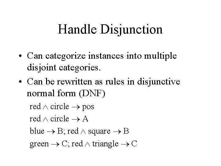
Handle Disjunction • Can categorize instances into multiple disjoint categories. • Can be rewritten as rules in disjunctive normal form (DNF) red Ù circle ® pos red Ù circle ® A blue ® B; red Ù square ® B green ® C; red Ù triangle ® C

Decision Tree Learning • Instances are represented as attribute value pairs. • Discrete values are simplest, thresholds on numerical features are also possible for splitting nodes. • Output is a discrete category. Real valued outputs are possible with additions (regression trees).

Decision Tree Learning cont. • Algorithms are efficient for processing large amounts of data. • Methods are available for handling noisy data (category and attribute noise). • Methods are available for handling missing attribute values.

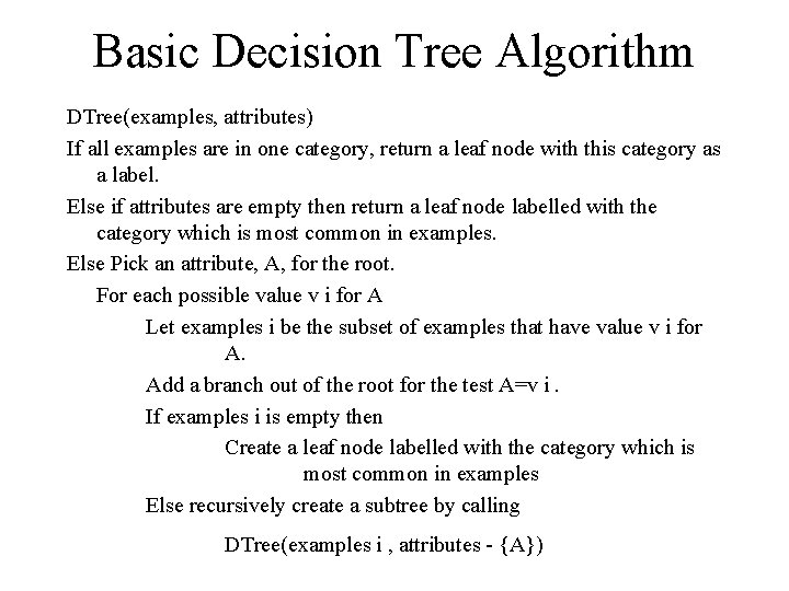
Basic Decision Tree Algorithm DTree(examples, attributes) If all examples are in one category, return a leaf node with this category as a label. Else if attributes are empty then return a leaf node labelled with the category which is most common in examples. Else Pick an attribute, A, for the root. For each possible value v i for A Let examples i be the subset of examples that have value v i for A. Add a branch out of the root for the test A=v i. If examples i is empty then Create a leaf node labelled with the category which is most common in examples Else recursively create a subtree by calling DTree(examples i , attributes {A})

Picking an Attribute to Split On • Goal is to have the resulting decision tree be as small as possible, following Occam's Razor. • Finding a minimal decision tree consistent with a set of data is NP hard. • Simple recursive algorithm does a greedy heuristic search for a fairly simple tree but cannot guarantee optimality.

What Is a Good Test? • Want a test which creates subsets which are relatively “pure” in one class so that they are closer to being leaf nodes. • There are various heuristics for picking a good test, the most popular one based on information gain (mutual information) originated with ID 3 system of Quinlan (1979)

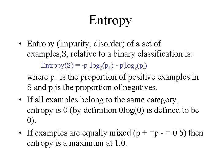
Entropy • Entropy (impurity, disorder) of a set of examples, S, relative to a binary classification is: Entropy(S) = p+log 2(p+) p log 2(p ) where p+ is the proportion of positive examples in S and p is the proportion of negatives. • If all examples belong to the same category, entropy is 0 (by definition 0 log(0) is defined to be 0). • If examples are equally mixed (p + =p = 0. 5) then entropy is a maximum at 1. 0.

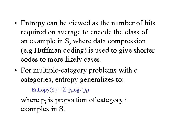
• Entropy can be viewed as the number of bits required on average to encode the class of an example in S, where data compression (e. g Huffman coding) is used to give shorter codes to more likely cases. • For multiple category problems with c categories, entropy generalizes to: Entropy(S) = pilog 2(pi) where pi is proportion of category i examples in S.

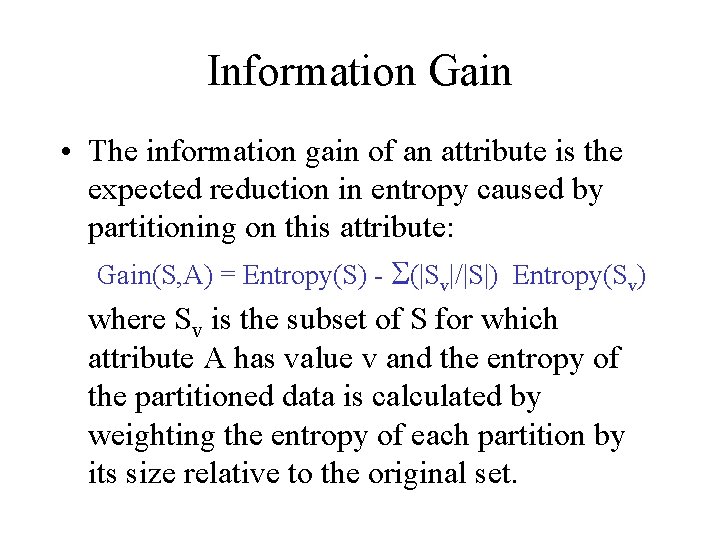
Information Gain • The information gain of an attribute is the expected reduction in entropy caused by partitioning on this attribute: Gain(S, A) = Entropy(S) (|Sv|/|S|) Entropy(Sv) where Sv is the subset of S for which attribute A has value v and the entropy of the partitioned data is calculated by weighting the entropy of each partition by its size relative to the original set.

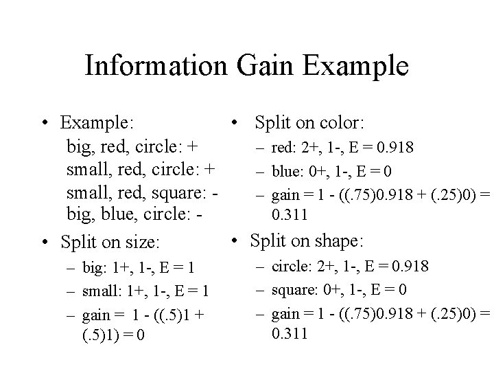
Information Gain Example • Example: • Split on color: big, red, circle: + – red: 2+, 1 , E = 0. 918 small, red, circle: + – blue: 0+, 1 , E = 0 small, red, square: – gain = 1 ((. 75)0. 918 + (. 25)0) = 0. 311 big, blue, circle: • Split on shape: • Split on size: – big: 1+, 1 , E = 1 – small: 1+, 1 , E = 1 – gain = 1 ((. 5)1 + (. 5)1) = 0 – circle: 2+, 1 , E = 0. 918 – square: 0+, 1 , E = 0 – gain = 1 ((. 75)0. 918 + (. 25)0) = 0. 311

Hypothesis Space in Decision Tree Induction • Conducts a search of the space of decision trees which can represent all possible discrete functions. • Creates a single discrete hypothesis consistent with the data, so there is no way to provide confidences or create useful queries.

Algorithm Characteristics • Performs hill climbing search so may find a locally optimal solution. Guaranteed to find a tree that fits any noise free training set, but it may not be the smallest. • Performs batch learning. Bases each decision on a batch of examples and can terminate early to avoid fitting noisy data.

Bias • Bias is for trees of minimal depth; however, greedy search introduces a complication that it may not find the minimal tree and positions features with high information gain high in the tree. • Implements a preference bias (search bias) as opposed to a restriction bias (language bias) like candidate elimination.

Simplicity • Occam's razor can be defended on the basis that there are relatively few simple hypotheses compared to complex ones, therefore, a simple hypothesis that is consistent with the data is less likely to be a statistical coincidence than finding a complex, consistent hypothesis. • However, – Simplicity is relative to the hypothesis language used. – This is an argument for any small hypothesis space and holds equally well for a small space of arcane complex hypotheses, e. g. decision trees with exactly 133 nodes where attributes along every branch are ordered alphabetically from root to leaf.

Overfitting • Learning a tree that classifies the training data perfectly may not lead to the tree with the best generalization performance since – There may be noise in the training data that the tree is fitting. – The algorithm might be making some decisions toward the leaves of the tree that are based on very little data and may not reflect reliable trends in the data. • A hypothesis, h, is said to overfit the training data if there exists another hypothesis, h’, such that h has smaller error than h’ on the training data but h’ has smaller error on the test data than h.

Overfitting and Noise • Category or attribute noise can cause overfitting. • Add noisy instance: – <<medium, green, circle>, +> (really ) • Noise can also cause directly conflicting examples with same description and different class. Impossible to fit this data and must label leaf with majority category. – <<big, red, circle>, > (really +) • Conflicting examples can also arise if attributes are incomplete and inadequate to discriminate the categories.

Avoiding Overfitting • Two basic approaches – Prepruning: Stop growing the tree at some point during construction when it is determined that there is not enough data to make reliable choices. – Postpruning: Grow the full tree and then remove nodes that seem to not have sufficient evidence.

Evaluating Subtrees to Prune • Cross validation: – Reserve some of the training data as a hold out set (validation set, tuning set) to evaluate utility of subtrees. • Statistical testing: – Perform some statistical test on the training data to determine if any observed regularity can be dismissed as likely to to random chance. • Minimum Description Length (MDL): – Determine if the additional complexity of the hypothesis is less complex than just explicitly remembering any exceptions.