EEL 4768 Computer Architecture Lecture 5 MIPS 64

EEL 4768 Computer Architecture Lecture 5: MIPS 64 Examples

Outline • Conversions • Floating-Point Arithmetic • Examples 2

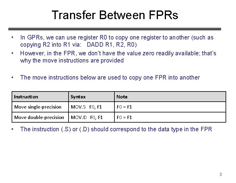
Transfer Between FPRs • • In GPRs, we can use register R 0 to copy one register to another (such as copying R 2 into R 1 via: DADD R 1, R 2, R 0) However, in the FPR, we don’t have the value zero readily available; that’s why the move instructions are provided The move instructions below are used to copy one FPR into another Instruction Syntax Note Move single-precision MOV. S F 0, F 1 F 0 = F 1 Move double-precision MOV. D F 0, F 1 F 0 = F 1 The instruction (. S) or (. D) should correspond to the data type in the FPR 3

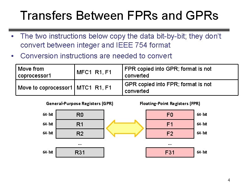
Transfers Between FPRs and GPRs • The two instructions below copy the data bit-by-bit; they don’t convert between integer and IEEE 754 format • Conversion instructions are needed to convert Move from coprocessor 1 MFC 1 R 1, F 1 FPR copied into GPR; format is not converted Move to coprocessor 1 MTC 1 R 1, F 1 GPR copied into FPR; format is not converted General-Purpose Registers (GPR) Floating-Point Registers (FPR) 64 -bit R 0 F 0 64 -bit R 1 F 1 64 -bit R 2 F 2 64 -bit … … R 31 F 31 64 -bit 4

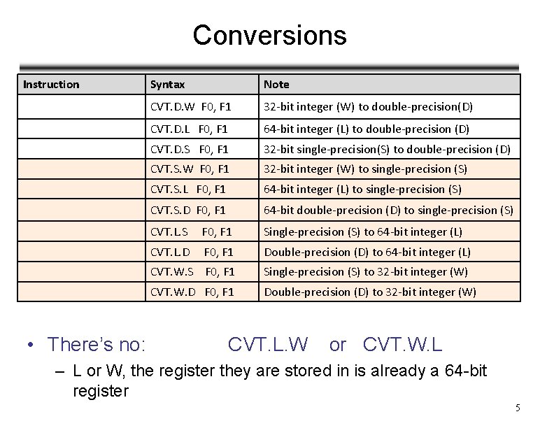
Conversions Instruction • There’s no: Syntax Note CVT. D. W F 0, F 1 32 -bit integer (W) to double-precision(D) CVT. D. L F 0, F 1 64 -bit integer (L) to double-precision (D) CVT. D. S F 0, F 1 32 -bit single-precision(S) to double-precision (D) CVT. S. W F 0, F 1 32 -bit integer (W) to single-precision (S) CVT. S. L F 0, F 1 64 -bit integer (L) to single-precision (S) CVT. S. D F 0, F 1 64 -bit double-precision (D) to single-precision (S) CVT. L. S F 0, F 1 Single-precision (S) to 64 -bit integer (L) CVT. L. D F 0, F 1 Double-precision (D) to 64 -bit integer (L) CVT. W. S F 0, F 1 Single-precision (S) to 32 -bit integer (W) CVT. W. D F 0, F 1 Double-precision (D) to 32 -bit integer (W) CVT. L. W or CVT. W. L – L or W, the register they are stored in is already a 64 -bit register 5

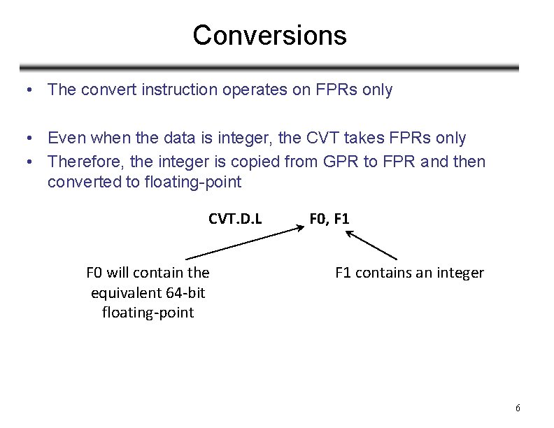
Conversions • The convert instruction operates on FPRs only • Even when the data is integer, the CVT takes FPRs only • Therefore, the integer is copied from GPR to FPR and then converted to floating-point CVT. D. L F 0 will contain the equivalent 64 -bit floating-point F 0, F 1 contains an integer 6

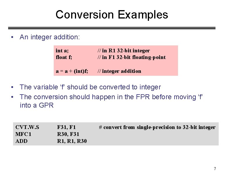
Conversion Examples • An integer addition: int a; float f; // in R 1 32 -bit integer // in F 1 32 -bit floating-point a = a + (int)f; // integer addition • The variable ‘f’ should be converted to integer • The conversion should happen in the FPR before moving ‘f’ into a GPR CVT. W. S MFC 1 ADD F 31, F 1 R 30, F 31 R 1, R 30 # convert from single-precision to 32 -bit integer 7

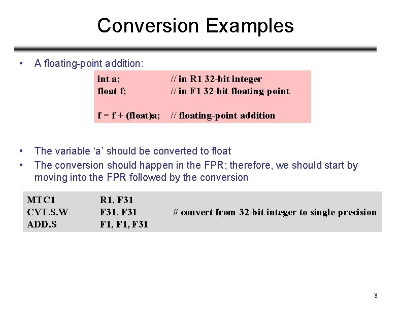
Conversion Examples • • • A floating-point addition: int a; float f; // in R 1 32 -bit integer // in F 1 32 -bit floating-point f = f + (float)a; // floating-point addition The variable ‘a’ should be converted to float The conversion should happen in the FPR; therefore, we should start by moving into the FPR followed by the conversion MTC 1 CVT. S. W ADD. S R 1, F 31, F 31 F 1, F 31 # convert from 32 -bit integer to single-precision 8

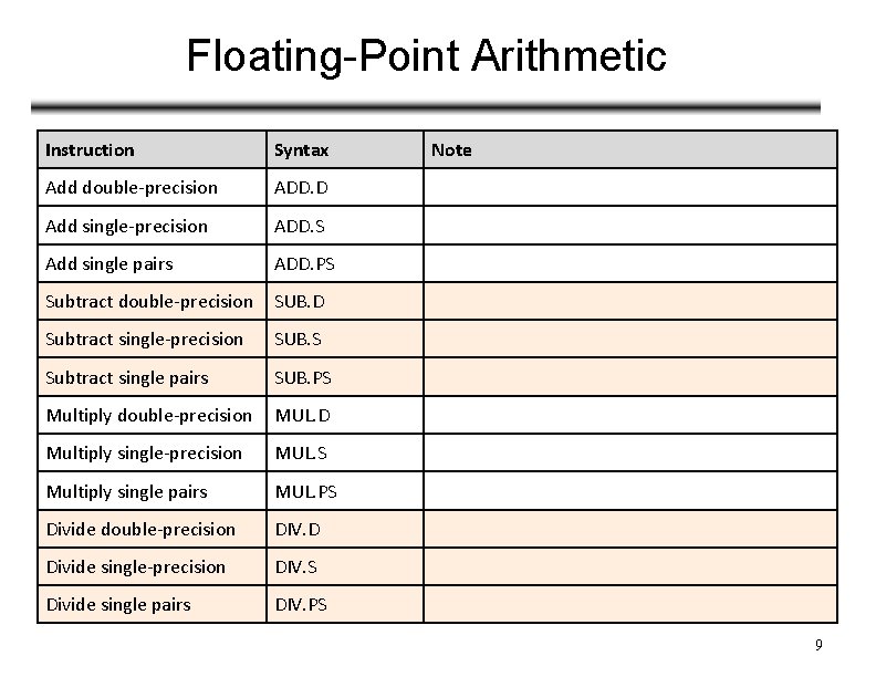
Floating-Point Arithmetic Instruction Syntax Add double-precision ADD. D Add single-precision ADD. S Add single pairs ADD. PS Subtract double-precision SUB. D Subtract single-precision SUB. S Subtract single pairs SUB. PS Multiply double-precision MUL. D Multiply single-precision MUL. S Multiply single pairs MUL. PS Divide double-precision DIV. D Divide single-precision DIV. S Divide single pairs DIV. PS Note 9

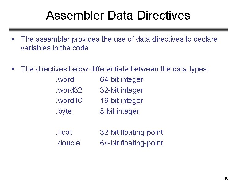
Assembler Data Directives • The assembler provides the use of data directives to declare variables in the code • The directives below differentiate between the data types: . word 64 -bit integer. word 32 32 -bit integer. word 16 16 -bit integer. byte 8 -bit integer. float. double 32 -bit floating-point 64 -bit floating-point 10

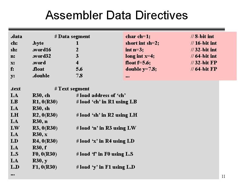
Assembler Data Directives char ch=1; short int sh=2; int n=3; long int x=4; float f=5. 6; double y=7. 8; . . data ch: sh: n: x: f: y: # Data segment. byte 1. word 16 2. word 32 3. word 4. float 5. 6. double 7. 8 . text LA LB LA LH LA LW LA LD LA L. S LA L. D. . . # Text segment R 30, ch # load address of ‘ch’ R 1, 0(R 30) # load ‘ch’ in R 1 using LB R 30, sh R 2, 0(R 30) # load ‘sh’ in R 2 using LH R 30, n R 3, 0(R 30) # load ‘n’ in R 3 using LW R 30, x R 4, 0(R 30) # load ‘x’ in R 4 using LD R 30, f F 0, 0(R 30) # load ‘f’ in F 0 using L. S R 30, y F 1, 0(R 30) # load ‘y’ in F 1 using L. D // 8 -bit int // 16 -bit int // 32 -bit int // 64 -bit int // 32 -bit FP // 64 -bit FP 11

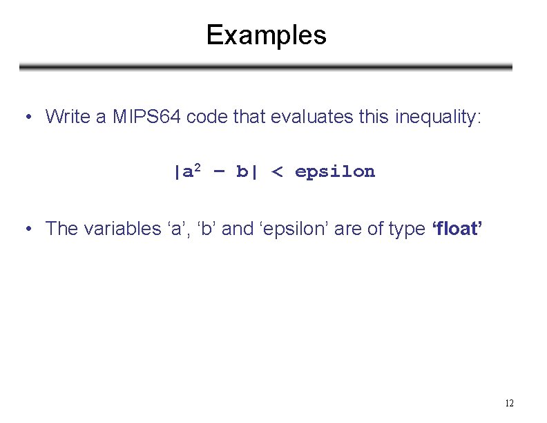
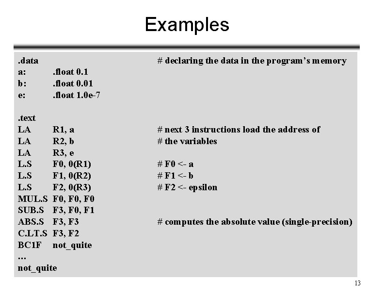
Examples • Write a MIPS 64 code that evaluates this inequality: |a 2 – b| < epsilon • The variables ‘a’, ‘b’ and ‘epsilon’ are of type ‘float’ 12

Examples. data a: b: e: # declaring the data in the program’s memory. float 0. 1. float 0. 01. float 1. 0 e-7 . text LA R 1, a LA R 2, b LA R 3, e L. S F 0, 0(R 1) L. S F 1, 0(R 2) L. S F 2, 0(R 3) MUL. S F 0, F 0 SUB. S F 3, F 0, F 1 ABS. S F 3, F 3 C. LT. S F 3, F 2 BC 1 F not_quite … not_quite # next 3 instructions load the address of # the variables # F 0 <- a # F 1 <- b # F 2 <- epsilon # computes the absolute value (single-precision) 13

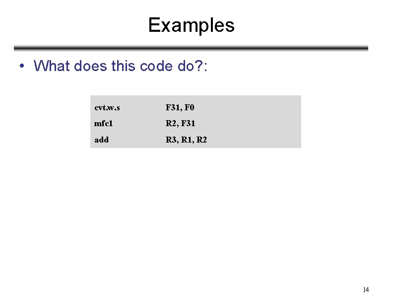
Examples • What does this code do? : cvt. w. s F 31, F 0 mfc 1 R 2, F 31 add R 3, R 1, R 2 14

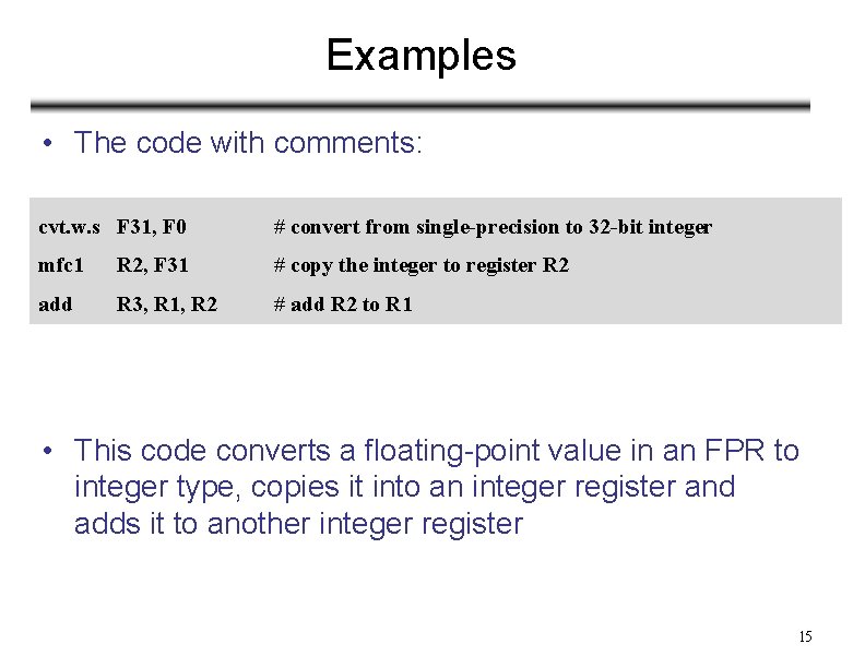
Examples • The code with comments: cvt. w. s F 31, F 0 # convert from single-precision to 32 -bit integer mfc 1 R 2, F 31 # copy the integer to register R 2 add R 3, R 1, R 2 # add R 2 to R 1 • This code converts a floating-point value in an FPR to integer type, copies it into an integer register and adds it to another integer register 15

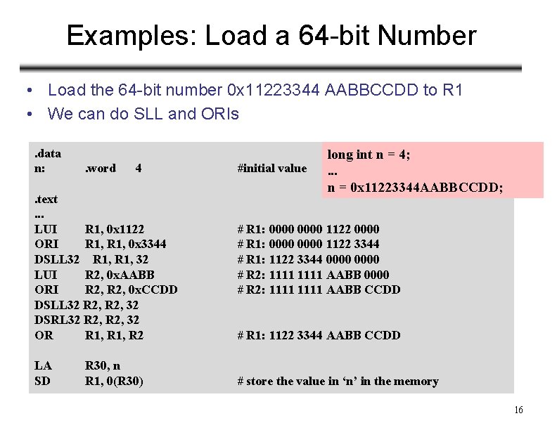
Examples: Load a 64 -bit Number • Load the 64 -bit number 0 x 11223344 AABBCCDD to R 1 • We can do SLL and ORIs. data n: . word 4 . text. . . LUI R 1, 0 x 1122 ORI R 1, 0 x 3344 DSLL 32 R 1, 32 LUI R 2, 0 x. AABB ORI R 2, 0 x. CCDD DSLL 32 R 2, 32 DSRL 32 R 2, 32 OR R 1, R 2 LA SD R 30, n R 1, 0(R 30) #initial value long int n = 4; . . . n = 0 x 11223344 AABBCCDD; # R 1: 0000 1122 0000 # R 1: 0000 1122 3344 # R 1: 1122 3344 0000 # R 2: 1111 AABB CCDD # R 1: 1122 3344 AABB CCDD # store the value in ‘n’ in the memory 16

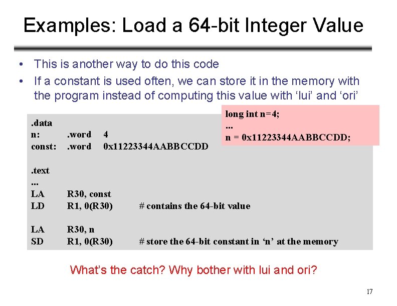
Examples: Load a 64 -bit Integer Value • This is another way to do this code • If a constant is used often, we can store it in the memory with the program instead of computing this value with ‘lui’ and ‘ori’ long int n=4; . . . n = 0 x 11223344 AABBCCDD; . data n: const: . word . text. . . LA LD R 30, const R 1, 0(R 30) # contains the 64 -bit value LA SD R 30, n R 1, 0(R 30) # store the 64 -bit constant in ‘n’ at the memory 4 0 x 11223344 AABBCCDD What’s the catch? Why bother with lui and ori? 17

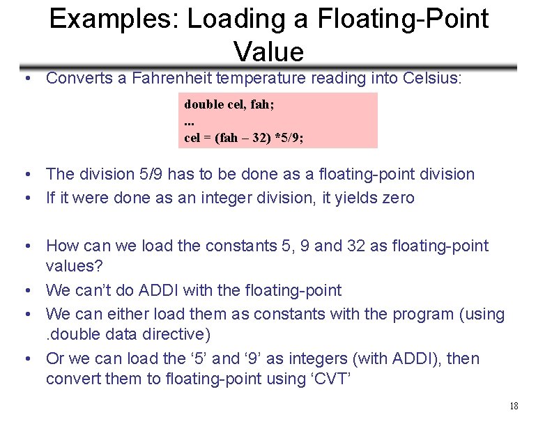
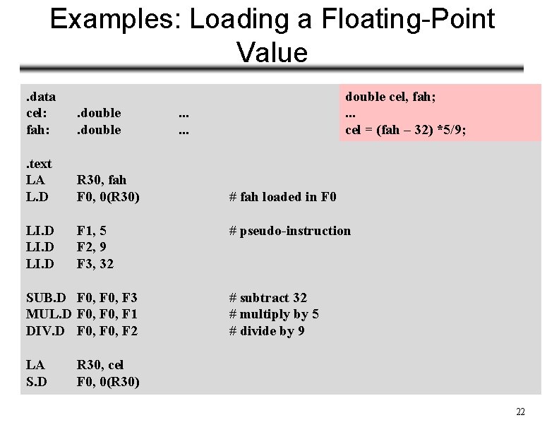
Examples: Loading a Floating-Point Value • Converts a Fahrenheit temperature reading into Celsius: double cel, fah; . . . cel = (fah – 32) *5/9; • The division 5/9 has to be done as a floating-point division • If it were done as an integer division, it yields zero • How can we load the constants 5, 9 and 32 as floating-point values? • We can’t do ADDI with the floating-point • We can either load them as constants with the program (using. double data directive) • Or we can load the ‘ 5’ and ‘ 9’ as integers (with ADDI), then convert them to floating-point using ‘CVT’ 18

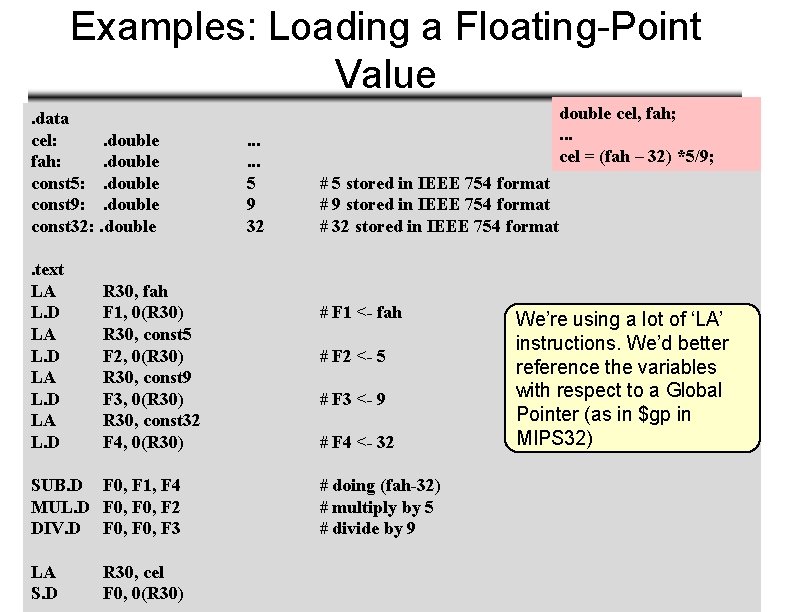
Examples: Loading a Floating-Point Value. data cel: . double fah: . double const 5: . double const 9: . double const 32: . double. text LA L. D R 30, fah F 1, 0(R 30) R 30, const 5 F 2, 0(R 30) R 30, const 9 F 3, 0(R 30) R 30, const 32 F 4, 0(R 30) SUB. D F 0, F 1, F 4 MUL. D F 0, F 2 DIV. D F 0, F 3 LA S. D R 30, cel F 0, 0(R 30) . . . 5 9 32 double cel, fah; . . . cel = (fah – 32) *5/9; # 5 stored in IEEE 754 format # 9 stored in IEEE 754 format # 32 stored in IEEE 754 format # F 1 <- fah # F 2 <- 5 # F 3 <- 9 # F 4 <- 32 We’re using a lot of ‘LA’ instructions. We’d better reference the variables with respect to a Global Pointer (as in $gp in MIPS 32) # doing (fah-32) # multiply by 5 # divide by 9 19

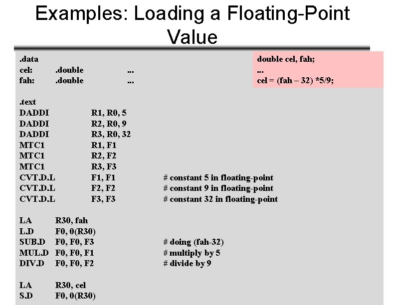
Examples: Loading a Floating-Point Value. data cel: fah: . text DADDI MTC 1 CVT. D. L . double cel, fah; . . . cel = (fah – 32) *5/9; . . . R 1, R 0, 5 R 2, R 0, 9 R 3, R 0, 32 R 1, F 1 R 2, F 2 R 3, F 3 F 1, F 1 F 2, F 2 F 3, F 3 LA L. D SUB. D MUL. D DIV. D R 30, fah F 0, 0(R 30) F 0, F 3 F 0, F 1 F 0, F 2 LA S. D R 30, cel F 0, 0(R 30) # constant 5 in floating-point # constant 9 in floating-point # constant 32 in floating-point # doing (fah-32) # multiply by 5 # divide by 9 20

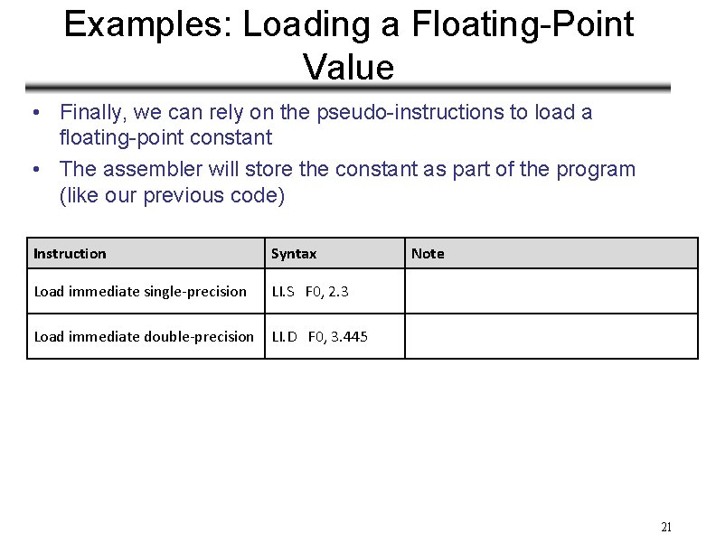
Examples: Loading a Floating-Point Value • Finally, we can rely on the pseudo-instructions to load a floating-point constant • The assembler will store the constant as part of the program (like our previous code) Instruction Syntax Load immediate single-precision LI. S F 0, 2. 3 Load immediate double-precision LI. D F 0, 3. 445 Note 21

Examples: Loading a Floating-Point Value. data cel: fah: . double . text LA L. D R 30, fah F 0, 0(R 30) LI. D F 1, 5 F 2, 9 F 3, 32 SUB. D F 0, F 3 MUL. D F 0, F 1 DIV. D F 0, F 2 LA S. D double cel, fah; . . . cel = (fah – 32) *5/9; . . . # fah loaded in F 0 # pseudo-instruction # subtract 32 # multiply by 5 # divide by 9 R 30, cel F 0, 0(R 30) 22

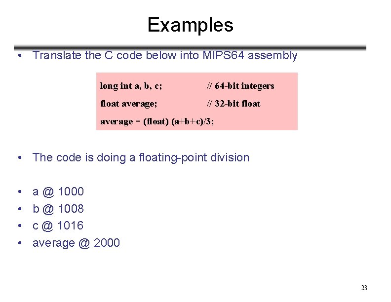
Examples • Translate the C code below into MIPS 64 assembly long int a, b, c; // 64 -bit integers float average; // 32 -bit float average = (float) (a+b+c)/3; • The code is doing a floating-point division • • a @ 1000 b @ 1008 c @ 1016 average @ 2000 23

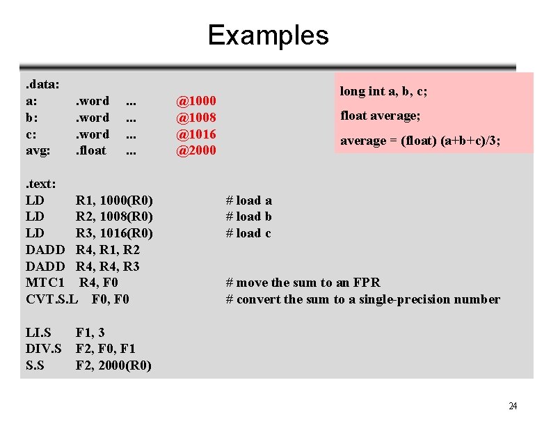
Examples. data: a: b: c: avg: . word. float . . . text: LD R 1, 1000(R 0) LD R 2, 1008(R 0) LD R 3, 1016(R 0) DADD R 4, R 1, R 2 DADD R 4, R 3 MTC 1 R 4, F 0 CVT. S. L F 0, F 0 long int a, b, c; @1000 @1008 @1016 @2000 float average; average = (float) (a+b+c)/3; # load a # load b # load c # move the sum to an FPR # convert the sum to a single-precision number LI. S F 1, 3 DIV. S F 2, F 0, F 1 S. S F 2, 2000(R 0) 24

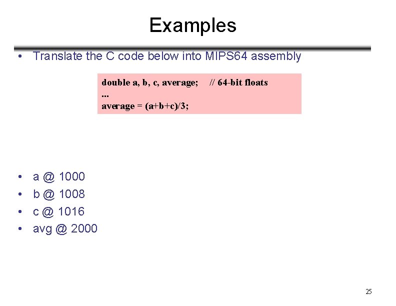
Examples • Translate the C code below into MIPS 64 assembly double a, b, c, average; . . . average = (a+b+c)/3; • • // 64 -bit floats a @ 1000 b @ 1008 c @ 1016 avg @ 2000 25

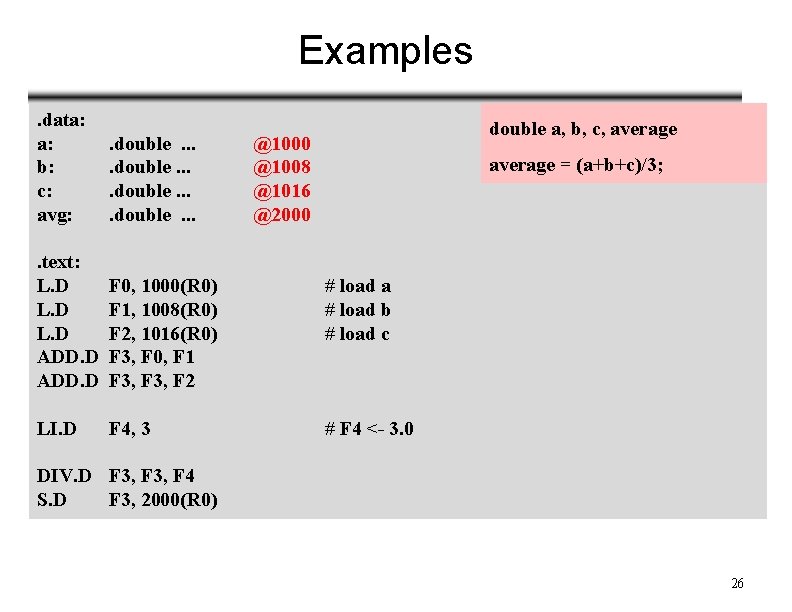
Examples. data: a: b: c: avg: . double. . . . text: L. D ADD. D F 0, 1000(R 0) F 1, 1008(R 0) F 2, 1016(R 0) F 3, F 0, F 1 F 3, F 2 # load a # load b # load c LI. D F 4, 3 # F 4 <- 3. 0 double a, b, c, average @1000 @1008 @1016 @2000 average = (a+b+c)/3; DIV. D F 3, F 4 S. D F 3, 2000(R 0) 26

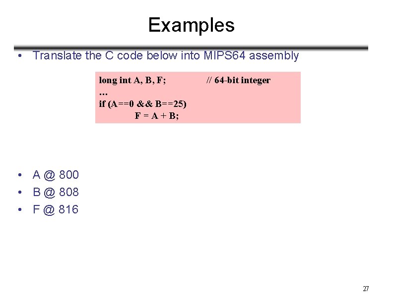
Examples • Translate the C code below into MIPS 64 assembly long int A, B, F; … if (A==0 && B==25) F = A + B; // 64 -bit integer • A @ 800 • B @ 808 • F @ 816 27

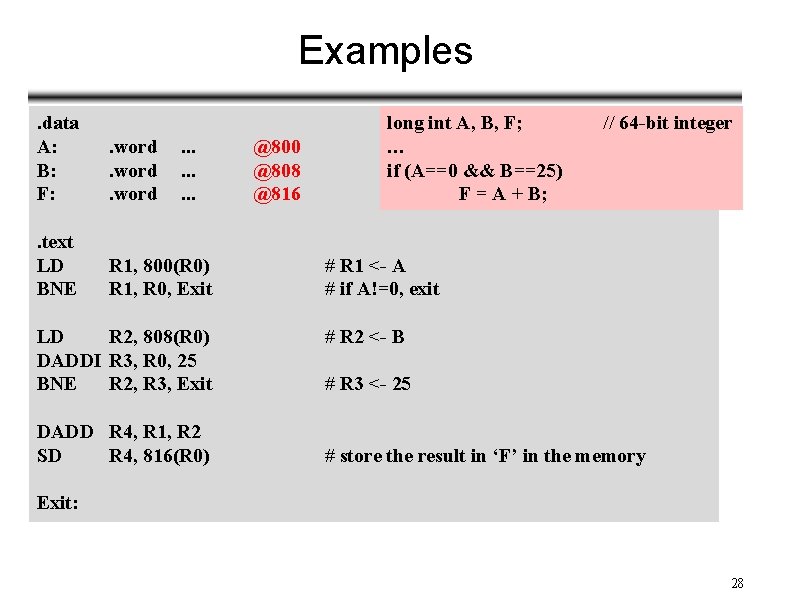
Examples. data A: B: F: . word . text LD BNE R 1, 800(R 0) R 1, R 0, Exit . . LD R 2, 808(R 0) DADDI R 3, R 0, 25 BNE R 2, R 3, Exit DADD R 4, R 1, R 2 SD R 4, 816(R 0) @800 @808 @816 long int A, B, F; … if (A==0 && B==25) F = A + B; // 64 -bit integer # R 1 <- A # if A!=0, exit # R 2 <- B # R 3 <- 25 # store the result in ‘F’ in the memory Exit: 28

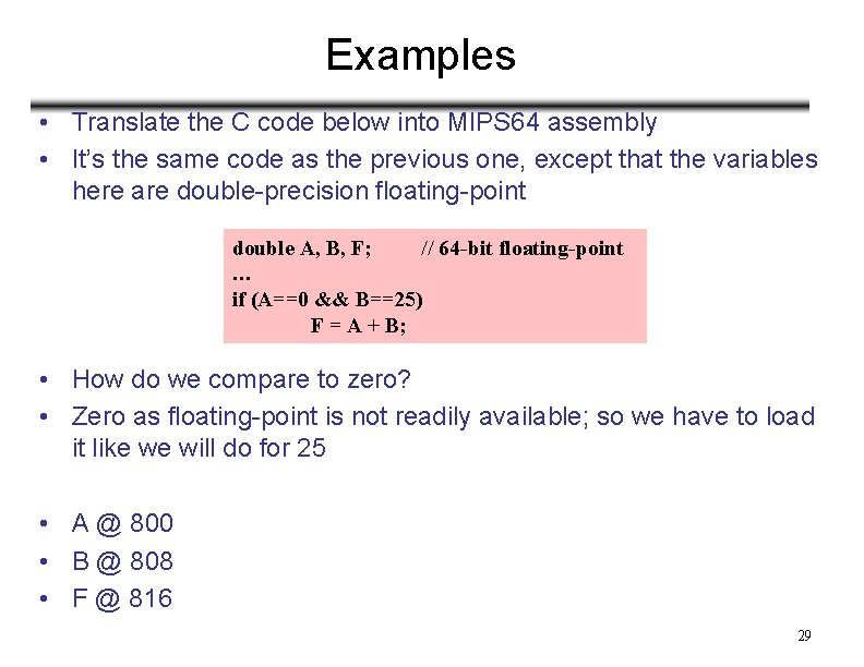
Examples • Translate the C code below into MIPS 64 assembly • It’s the same code as the previous one, except that the variables here are double-precision floating-point double A, B, F; // 64 -bit floating-point … if (A==0 && B==25) F = A + B; • How do we compare to zero? • Zero as floating-point is not readily available; so we have to load it like we will do for 25 • A @ 800 • B @ 808 • F @ 816 29

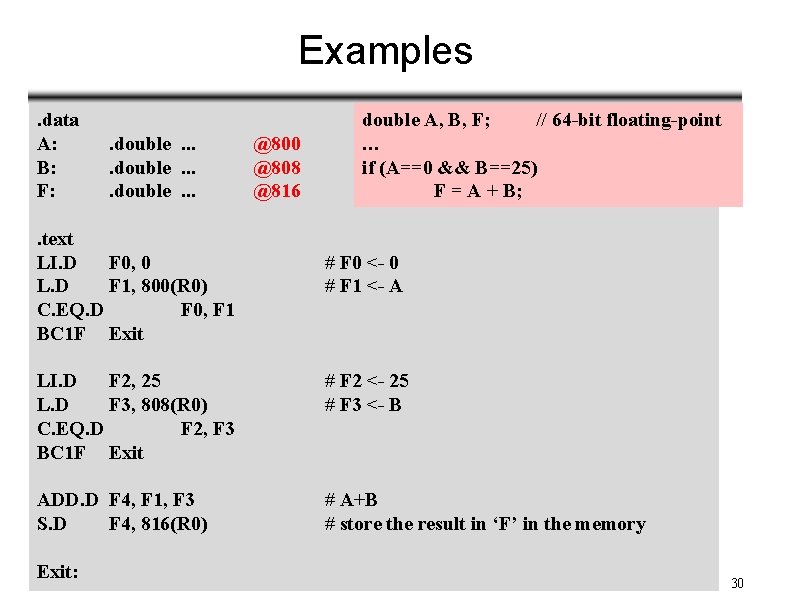
Examples. data A: B: F: . double. . text LI. D F 0, 0 L. D F 1, 800(R 0) C. EQ. D F 0, F 1 BC 1 F Exit @800 @808 @816 double A, B, F; // 64 -bit floating-point … if (A==0 && B==25) F = A + B; # F 0 <- 0 # F 1 <- A LI. D F 2, 25 L. D F 3, 808(R 0) C. EQ. D F 2, F 3 BC 1 F Exit # F 2 <- 25 # F 3 <- B ADD. D F 4, F 1, F 3 S. D F 4, 816(R 0) # A+B # store the result in ‘F’ in the memory Exit: 30

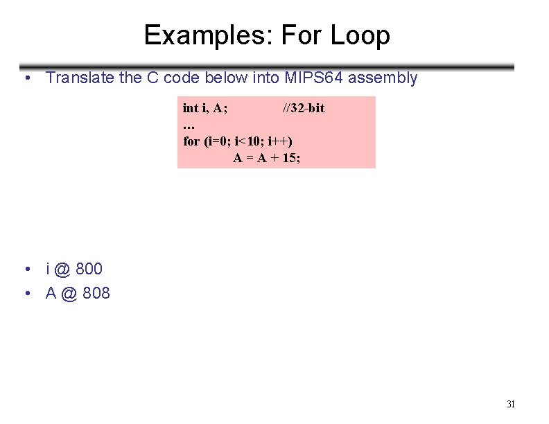
Examples: For Loop • Translate the C code below into MIPS 64 assembly int i, A; //32 -bit … for (i=0; i<10; i++) A = A + 15; • i @ 800 • A @ 808 31

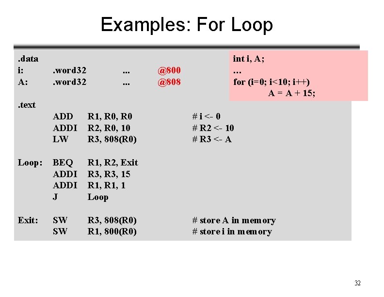
Examples: For Loop. data i: A: . word 32 . . . @800 @808 int i, A; … for (i=0; i<10; i++) A = A + 15; . text ADDI LW R 1, R 0 R 2, R 0, 10 R 3, 808(R 0) Loop: BEQ ADDI J R 1, R 2, Exit R 3, 15 R 1, 1 Loop Exit: SW SW R 3, 808(R 0) R 1, 800(R 0) # i <- 0 # R 2 <- 10 # R 3 <- A # store A in memory # store i in memory 32

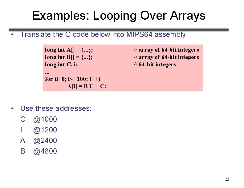
Examples: Looping Over Arrays • Translate the C code below into MIPS 64 assembly long int A[] = {. . . }; long int B[] = {. . . }; long int C, i; . . . for (i=0; i<=100; i++) A[i] = B[i] + C; // array of 64 -bit integers // 64 -bit integers • Use these addresses: C @1000 i @1200 A @2400 B @4800 33

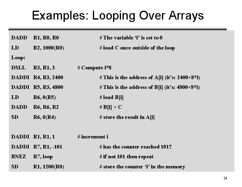
Examples: Looping Over Arrays DADD R 1, R 0 # The variable ‘i’ is set to 0 LD R 2, 1000(R 0) # load C once outside of the loop Loop: DSLL R 3, R 1, 3 # Compute i*8 DADDI R 4, R 3, 2400 # This is the address of A[i] (it’s: 2400+8*i) DADDI R 5, R 3, 4800 # This is the address of B[i] (it’s: 4800+8*i) LD R 6, 0(R 5) # load B[i] DADD R 6, R 2 # B[i] + C SD R 6, 0(R 4) # store the result in A[i] DADDI R 1, 1 # increment i DADDI R 7, R 1, -101 # has the counter reached 101? BNEZ R 7, loop # if not 101 then repeat SD R 1, 1200(R 0) # store the counter ‘i’ in the memory 34

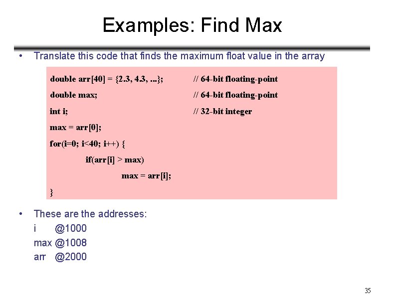
Examples: Find Max • Translate this code that finds the maximum float value in the array double arr[40] = {2. 3, 4. 3, . . . }; // 64 -bit floating-point double max; // 64 -bit floating-point i; // 32 -bit integer max = arr[0]; for(i=0; i<40; i++) { if(arr[i] > max) max = arr[i]; } • These are the addresses: i @1000 max @1008 arr @2000 35

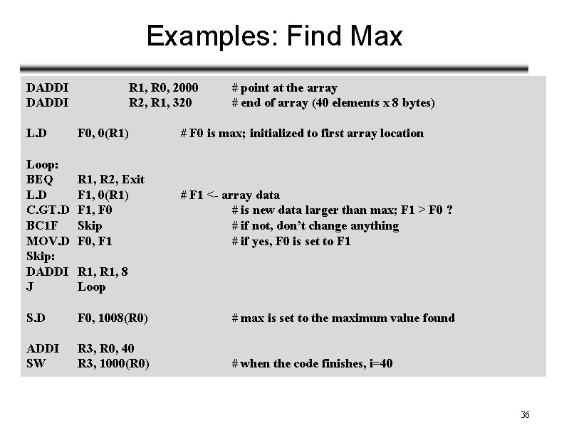
Examples: Find Max DADDI L. D Loop: BEQ L. D C. GT. D BC 1 F MOV. D Skip: DADDI J R 1, R 0, 2000 R 2, R 1, 320 # point at the array # end of array (40 elements x 8 bytes) F 0, 0(R 1) # F 0 is max; initialized to first array location R 1, R 2, Exit F 1, 0(R 1) F 1, F 0 Skip F 0, F 1 # F 1 <- array data # is new data larger than max; F 1 > F 0 ? # if not, don’t change anything # if yes, F 0 is set to F 1 R 1, 8 Loop S. D F 0, 1008(R 0) # max is set to the maximum value found ADDI SW R 3, R 0, 40 R 3, 1000(R 0) # when the code finishes, i=40 36

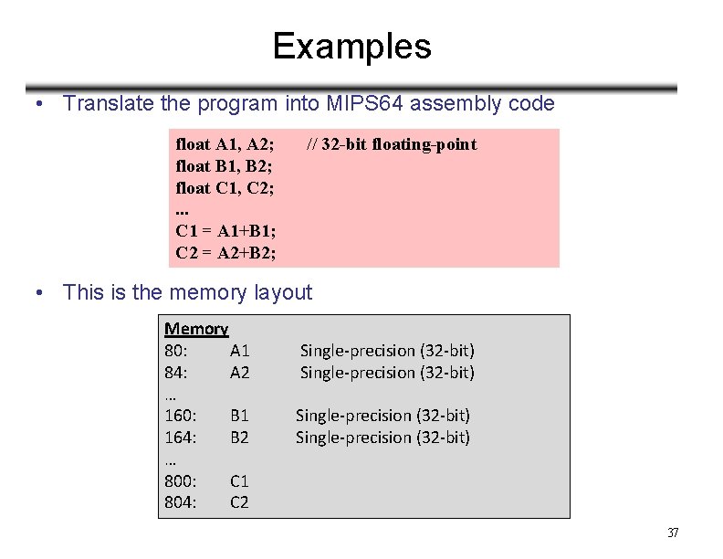
Examples • Translate the program into MIPS 64 assembly code float A 1, A 2; float B 1, B 2; float C 1, C 2; . . . C 1 = A 1+B 1; C 2 = A 2+B 2; // 32 -bit floating-point • This is the memory layout Memory 80: A 1 84: A 2 … 160: B 1 164: B 2 … 800: C 1 804: C 2 Single-precision (32 -bit) 37

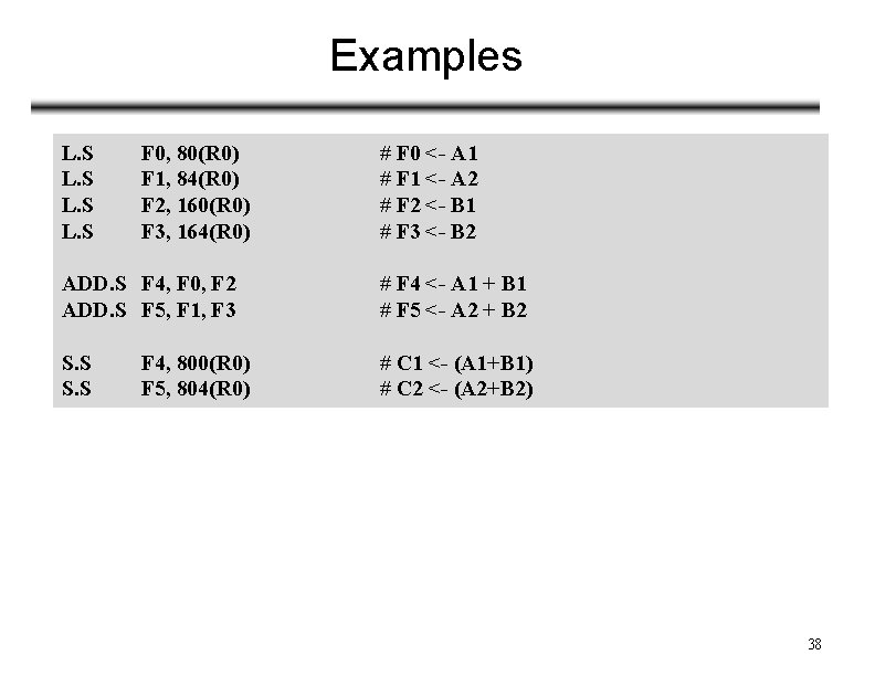
Examples L. S F 0, 80(R 0) F 1, 84(R 0) F 2, 160(R 0) F 3, 164(R 0) # F 0 <- A 1 # F 1 <- A 2 # F 2 <- B 1 # F 3 <- B 2 ADD. S F 4, F 0, F 2 ADD. S F 5, F 1, F 3 # F 4 <- A 1 + B 1 # F 5 <- A 2 + B 2 S. S # C 1 <- (A 1+B 1) # C 2 <- (A 2+B 2) F 4, 800(R 0) F 5, 804(R 0) 38

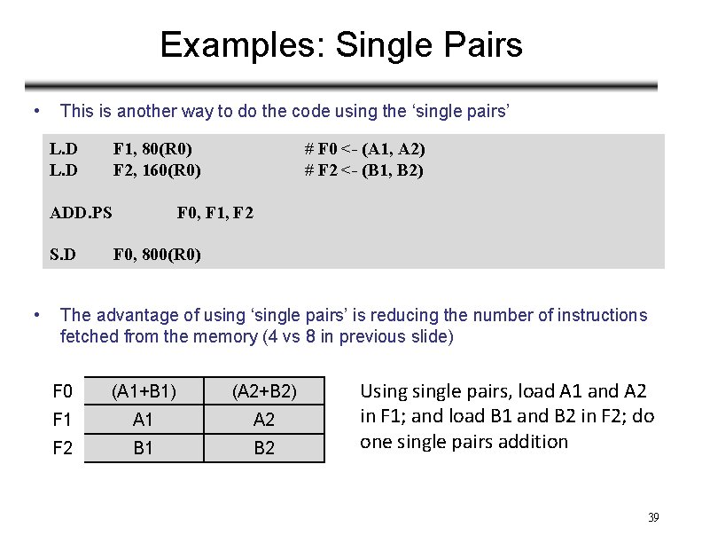
Examples: Single Pairs • This is another way to do the code using the ‘single pairs’ L. D F 1, 80(R 0) F 2, 160(R 0) ADD. PS S. D • # F 0 <- (A 1, A 2) # F 2 <- (B 1, B 2) F 0, F 1, F 2 F 0, 800(R 0) The advantage of using ‘single pairs’ is reducing the number of instructions fetched from the memory (4 vs 8 in previous slide) F 0 (A 1+B 1) (A 2+B 2) F 1 A 2 F 2 B 1 B 2 Usingle pairs, load A 1 and A 2 in F 1; and load B 1 and B 2 in F 2; do one single pairs addition 39

Readings • H&P CA – App K 40