EE 350 ECE 490 Analog Communication Systems Ch

- Slides: 48
EE 350 / ECE 490 Analog Communication Systems Ch. 5 – Frequency Modulation (FM) Transmission R. Munden - Fairfield University 2/23/2010 1
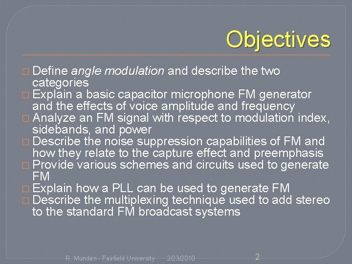
Objectives � Define angle modulation and describe the two categories � Explain a basic capacitor microphone FM generator and the effects of voice amplitude and frequency � Analyze an FM signal with respect to modulation index, sidebands, and power � Describe the noise suppression capabilities of FM and how they relate to the capture effect and preemphasis � Provide various schemes and circuits used to generate FM � Explain how a PLL can be used to generate FM � Describe the multiplexing technique used to add stereo to the standard FM broadcast systems R. Munden - Fairfield University 2/23/2010 2
5 -1 Angle Modulation � FM First postulated in 1931, first implemented by Major E. H. Armstrong in 1936, broadcast began in 1939. � Phase Modulation (PM) – phase angle of carrier varies with intelligence amplitude � Frequency Modulation (FM) – frequency of carrier varies with intelligence amplitude. � FM used for transmission, PM used to generate FM R. Munden - Fairfield University 2/23/2010 3
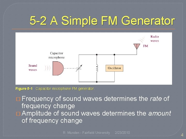
5 -2 A Simple FM Generator Figure 5 -1 Capacitor microphone FM generator. � Frequency of sound waves determines the rate of frequency change � Amplitude of sound waves determines the amount of frequency change R. Munden - Fairfield University 2/23/2010 4
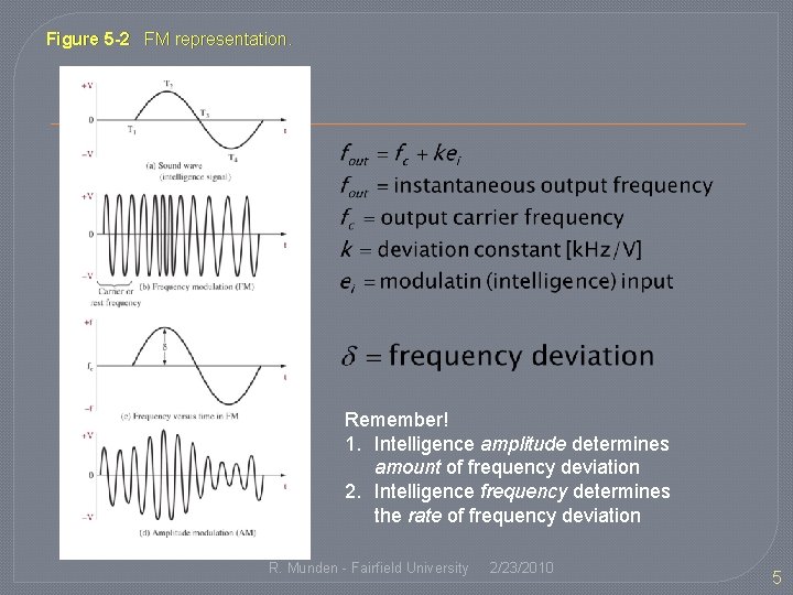
Figure 5 -2 FM representation. Remember! 1. Intelligence amplitude determines amount of frequency deviation 2. Intelligence frequency determines the rate of frequency deviation R. Munden - Fairfield University 2/23/2010 5
5 -3 FM Analysis � For PM � mp is the modulation index for PM � For FM � mf is the modulation index for FM R. Munden - Fairfield University 2/23/2010 6
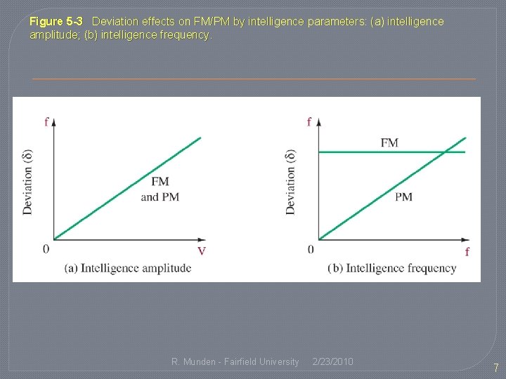
Figure 5 -3 Deviation effects on FM/PM by intelligence parameters: (a) intelligence amplitude; (b) intelligence frequency. R. Munden - Fairfield University 2/23/2010 7
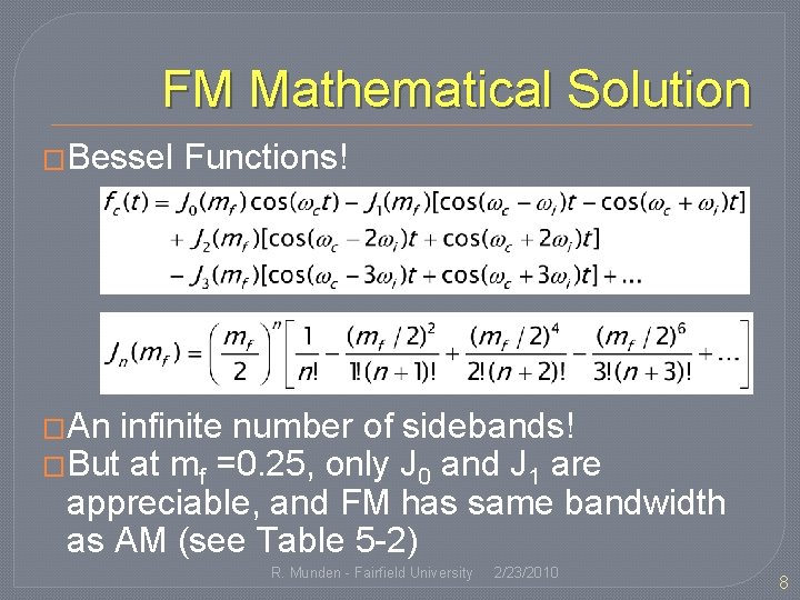
FM Mathematical Solution �Bessel Functions! �An infinite number of sidebands! �But at mf =0. 25, only J 0 and J 1 are appreciable, and FM has same bandwidth as AM (see Table 5 -2) R. Munden - Fairfield University 2/23/2010 8
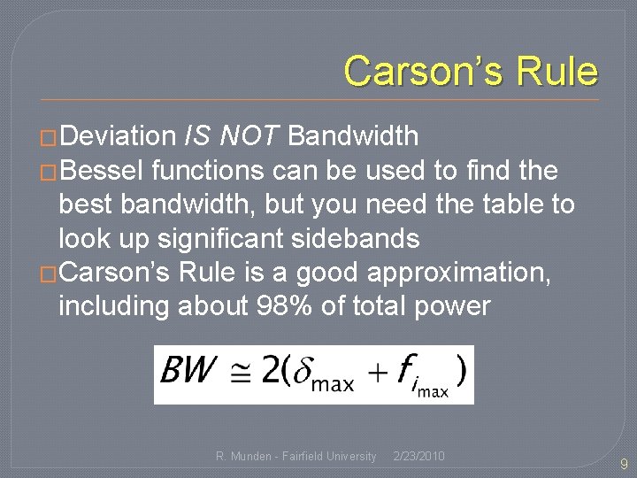
Carson’s Rule �Deviation IS NOT Bandwidth �Bessel functions can be used to find the best bandwidth, but you need the table to look up significant sidebands �Carson’s Rule is a good approximation, including about 98% of total power R. Munden - Fairfield University 2/23/2010 9
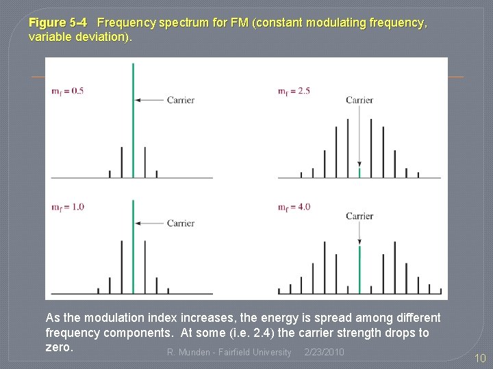
Figure 5 -4 Frequency spectrum for FM (constant modulating frequency, variable deviation). As the modulation index increases, the energy is spread among different frequency components. At some (i. e. 2. 4) the carrier strength drops to zero. R. Munden - Fairfield University 2/23/2010 10
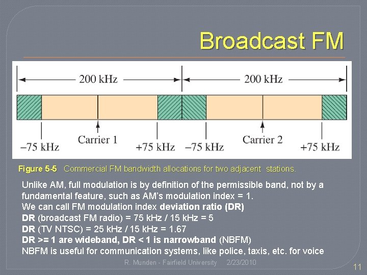
Broadcast FM Figure 5 -5 Commercial FM bandwidth allocations for two adjacent stations. Unlike AM, full modulation is by definition of the permissible band, not by a fundamental feature, such as AM’s modulation index = 1. We can call FM modulation index deviation ratio (DR) DR (broadcast FM radio) = 75 k. Hz / 15 k. Hz = 5 DR (TV NTSC) = 25 k. Hz / 15 k. Hz = 1. 67 DR >= 1 are wideband, DR < 1 is narrowband (NBFM) NBFM is useful for communication systems, like police, taxis, etc. for voice R. Munden - Fairfield University 2/23/2010 11
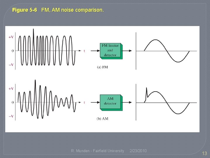
5 -4 Noise Suppression �Since noise changes the amplitude of the signal, this affects the intelligence in AM, resulting in noise �In FM, the amplitude is constant, so a spike in amplitude due to noise can be removed by a limiter R. Munden - Fairfield University 2/23/2010 12
Figure 5 -6 FM, AM noise comparison. R. Munden - Fairfield University 2/23/2010 13
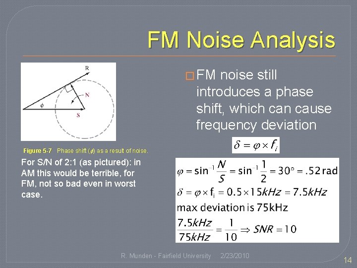
FM Noise Analysis � FM noise still introduces a phase shift, which can cause frequency deviation Figure 5 -7 Phase shift ( ) as a result of noise. For S/N of 2: 1 (as pictured): in AM this would be terrible, for FM, not so bad even in worst case. R. Munden - Fairfield University 2/23/2010 14
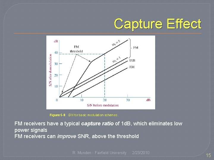
Capture Effect Figure 5 -8 S/N for basic modulation schemes. FM receivers have a typical capture ratio of 1 d. B, which eliminates low power signals FM receivers can improve SNR, above threshold R. Munden - Fairfield University 2/23/2010 15
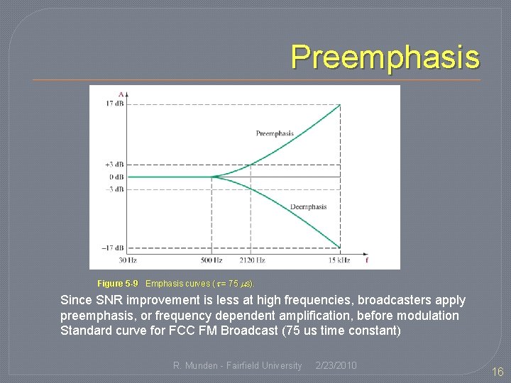
Preemphasis Figure 5 -9 Emphasis curves ( = 75 s). Since SNR improvement is less at high frequencies, broadcasters apply preemphasis, or frequency dependent amplification, before modulation Standard curve for FCC FM Broadcast (75 us time constant) R. Munden - Fairfield University 2/23/2010 16
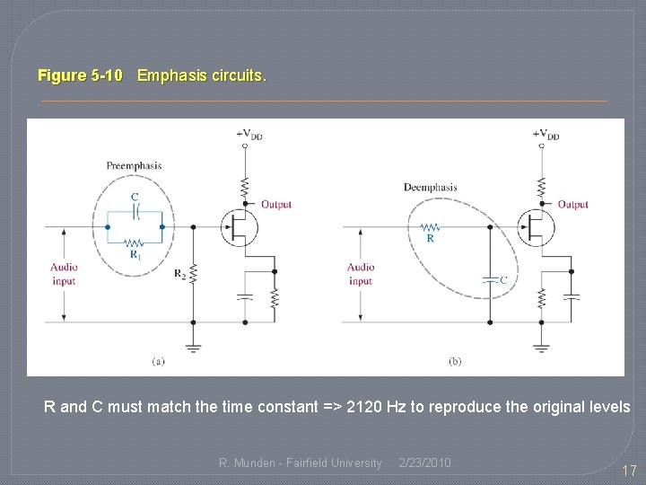
Figure 5 -10 Emphasis circuits. R and C must match the time constant => 2120 Hz to reproduce the original levels R. Munden - Fairfield University 2/23/2010 17
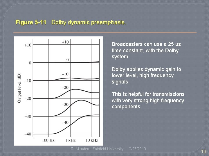
Figure 5 -11 Dolby dynamic preemphasis. Broadcasters can use a 25 us time constant, with the Dolby system Dolby applies dynamic gain to lower level, high frequency signals This is helpful for transmissions with very strong high frequency components R. Munden - Fairfield University 2/23/2010 18
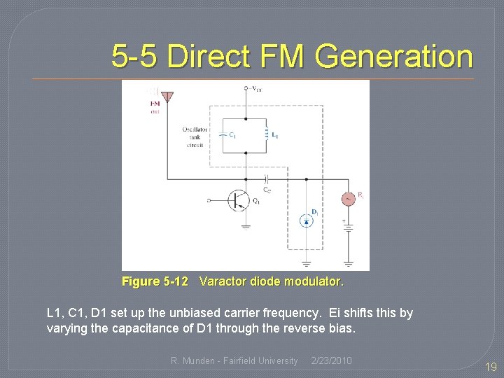
5 -5 Direct FM Generation Figure 5 -12 Varactor diode modulator. L 1, C 1, D 1 set up the unbiased carrier frequency. Ei shifts this by varying the capacitance of D 1 through the reverse bias. R. Munden - Fairfield University 2/23/2010 19
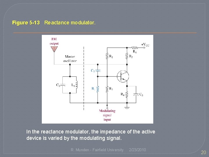
Figure 5 -13 Reactance modulator. In the reactance modulator, the impedance of the active device is varied by the modulating signal. R. Munden - Fairfield University 2/23/2010 20
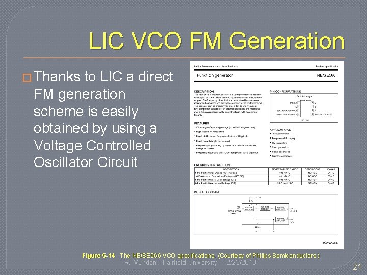
LIC VCO FM Generation � Thanks to LIC a direct FM generation scheme is easily obtained by using a Voltage Controlled Oscillator Circuit Figure 5 -14 The NE/SE 566 VCO specifications. (Courtesy of Philips Semiconductors. ) R. Munden - Fairfield University 2/23/2010 21
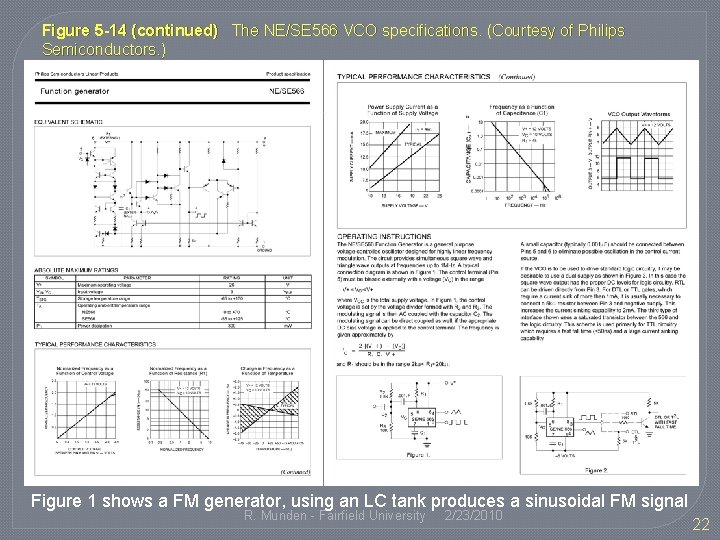
Figure 5 -14 (continued) The NE/SE 566 VCO specifications. (Courtesy of Philips Semiconductors. ) Figure 1 shows a FM generator, using an LC tank produces a sinusoidal FM signal R. Munden - Fairfield University 2/23/2010 22
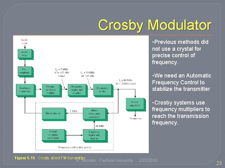
Crosby Modulator • Previous methods did not use a crystal for precise control of frequency. • We need an Automatic Frequency Control to stabilize the transmitter • Crosby systems use frequency multipliers to reach the transmission frequency. Figure 5 -15 Crosby direct FM transmitter. R. Munden - Fairfield University 2/23/2010 23
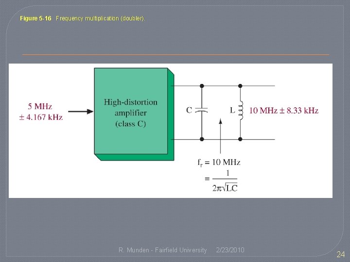
Figure 5 -16 Frequency multiplication (doubler). R. Munden - Fairfield University 2/23/2010 24
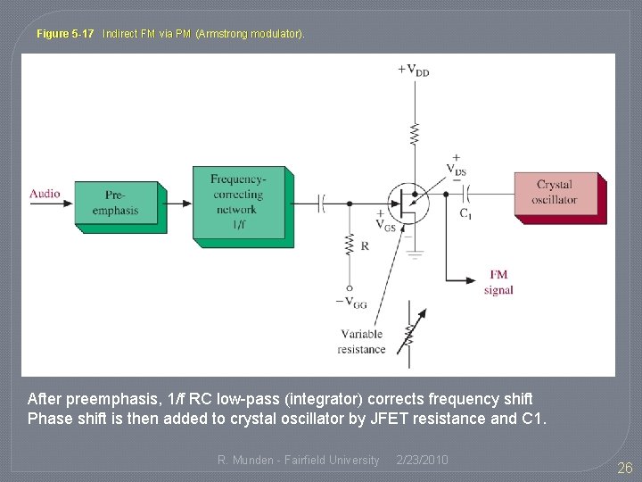
5 -6 Indirect FM Generation �Armstrong type modulator �Directly modulates the crystal oscillator by phase modulation (which indirectly varies the frequency) �Matches accuracy of crystal without AFC or degradation of Crosby systems R. Munden - Fairfield University 2/23/2010 25
Figure 5 -17 Indirect FM via PM (Armstrong modulator). After preemphasis, 1/f RC low-pass (integrator) corrects frequency shift Phase shift is then added to crystal oscillator by JFET resistance and C 1. R. Munden - Fairfield University 2/23/2010 26
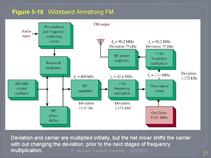
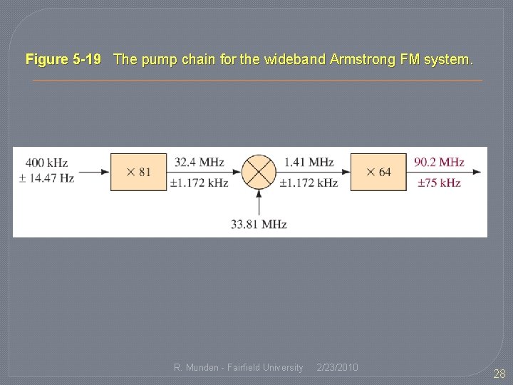
Figure 5 -18 Wideband Armstrong FM. Deviation and carrier are multiplied initially, but the het mixer shifts the carrier with out changing the deviation, prior to the next stages of frequency R. Munden - Fairfield University 2/23/2010 multiplication. 27
Figure 5 -19 The pump chain for the wideband Armstrong FM system. R. Munden - Fairfield University 2/23/2010 28
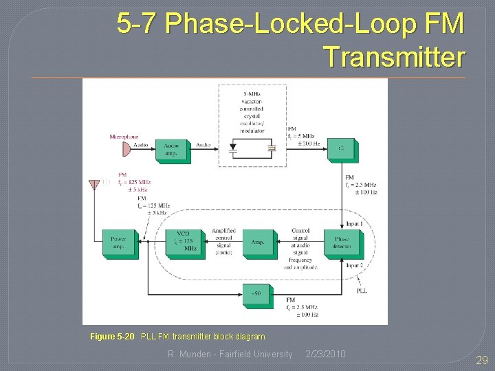
5 -7 Phase-Locked-Loop FM Transmitter Figure 5 -20 PLL FM transmitter block diagram. R. Munden - Fairfield University 2/23/2010 29
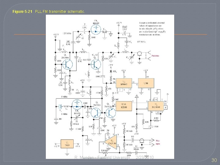
Figure 5 -21 PLL FM transmitter schematic. R. Munden - Fairfield University 2/23/2010 30
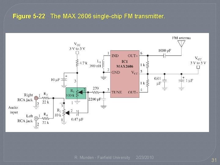
Figure 5 -22 The MAX 2606 single-chip FM transmitter. R. Munden - Fairfield University 2/23/2010 31
5 -8 Stereo FM �Information is doubled, so either time or bandwidth must be doubled (Hartley’s law) �Using Frequency Multiplexing avoids this problem R. Munden - Fairfield University 2/23/2010 32
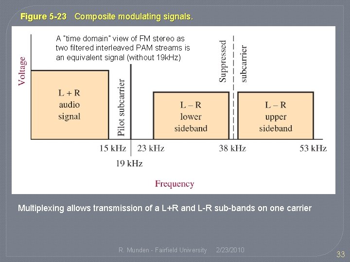
Figure 5 -23 Composite modulating signals. A ”time domain” view of FM stereo as two filtered interleaved PAM streams is an equivalent signal (without 19 k. Hz) Multiplexing allows transmission of a L+R and L-R sub-bands on one carrier R. Munden - Fairfield University 2/23/2010 33
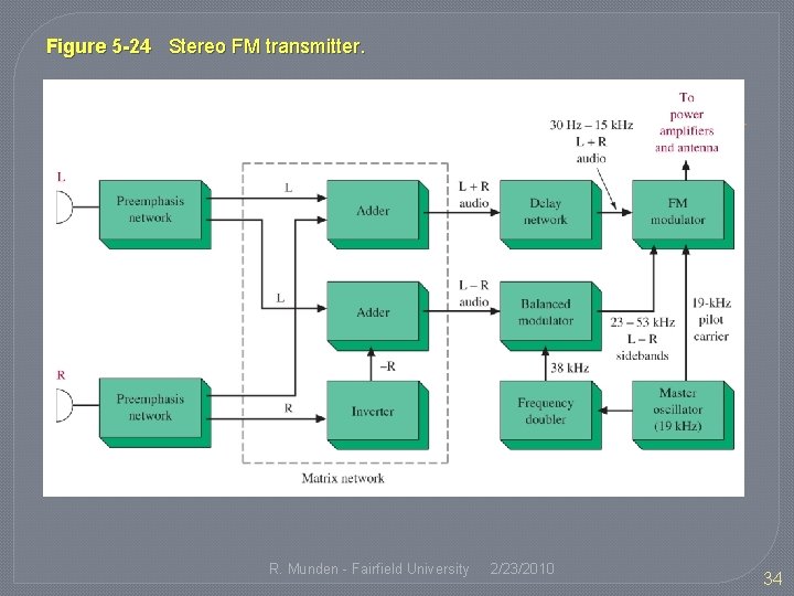
Figure 5 -24 Stereo FM transmitter. R. Munden - Fairfield University 2/23/2010 34
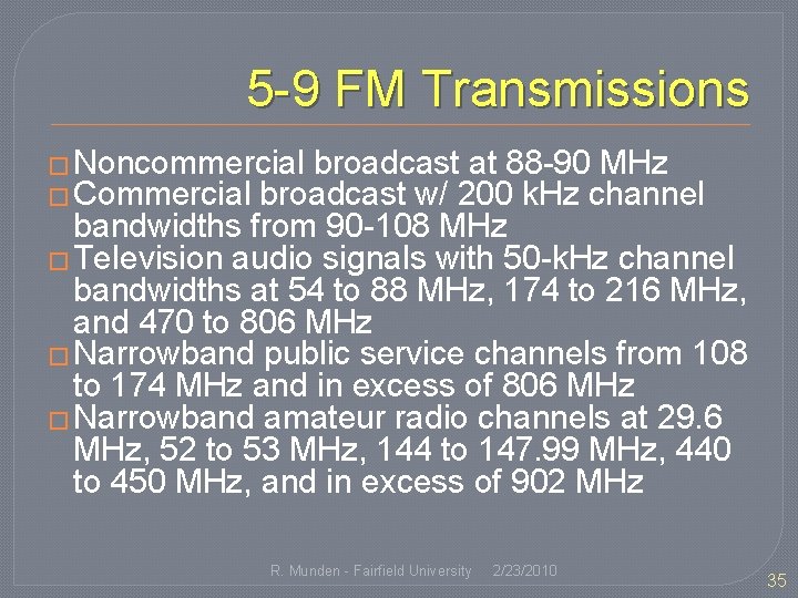
5 -9 FM Transmissions � Noncommercial broadcast at 88 -90 MHz � Commercial broadcast w/ 200 k. Hz channel bandwidths from 90 -108 MHz � Television audio signals with 50 -k. Hz channel bandwidths at 54 to 88 MHz, 174 to 216 MHz, and 470 to 806 MHz � Narrowband public service channels from 108 to 174 MHz and in excess of 806 MHz � Narrowband amateur radio channels at 29. 6 MHz, 52 to 53 MHz, 144 to 147. 99 MHz, 440 to 450 MHz, and in excess of 902 MHz R. Munden - Fairfield University 2/23/2010 35
Practical FM Transmission �Above 30 MHz due to ionosphere �Line-of-sight transmission (range of 70 – 80 miles) �Superior noise over SSB / AM �Uses low-level modulation and Class C power amplifiers for efficient transmission R. Munden - Fairfield University 2/23/2010 36
5 -10 Troubleshooting �Automotive Mobile �Fixed Base Station �Handheld portable �Both Wideband (broadcast) and Narrowband (communications) R. Munden - Fairfield University 2/23/2010 37
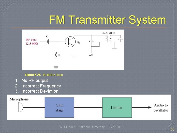
FM Transmitter System Figure 5 -25 Multiplier stage. 1. No RF output 2. Incorrect Frequency 3. Incorrect Deviation R. Munden - Fairfield University 2/23/2010 38
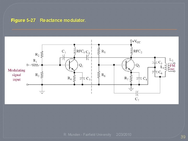
Figure 5 -27 Reactance modulator. R. Munden - Fairfield University 2/23/2010 39
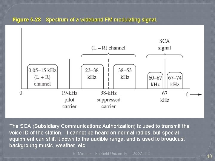
Figure 5 -28 Spectrum of a wideband FM modulating signal. The SCA (Subsidiary Communications Authorization) is used to transmit the voice ID of the station. It cannot be heard on normal radios, but special equipment can shift it down to the audible range, and is used to broadcast backgroung music, weather, etc. R. Munden - Fairfield University 2/23/2010 40
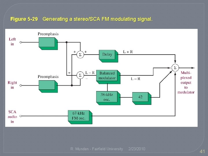
Figure 5 -29 Generating a stereo/SCA FM modulating signal. R. Munden - Fairfield University 2/23/2010 41
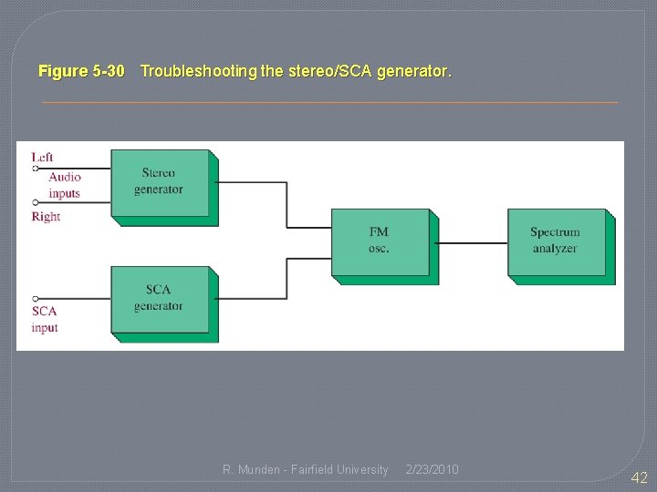
Figure 5 -30 Troubleshooting the stereo/SCA generator. R. Munden - Fairfield University 2/23/2010 42
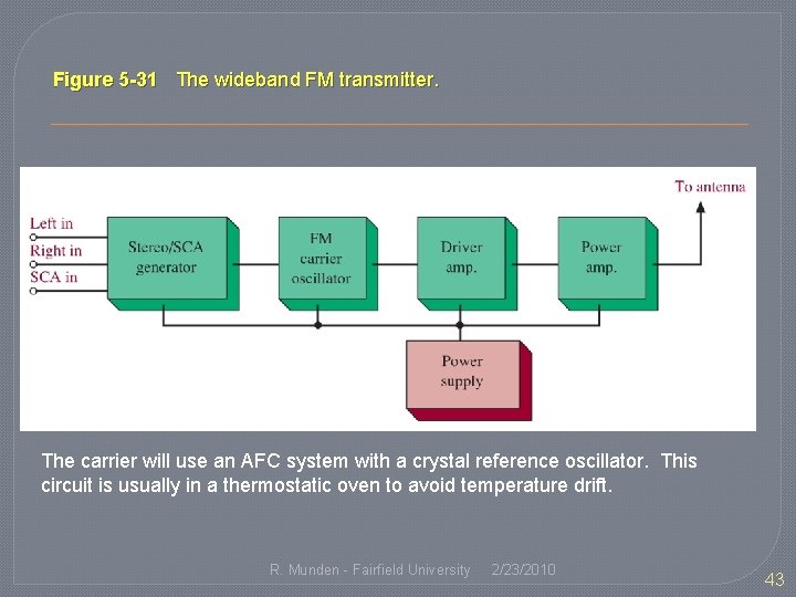
Figure 5 -31 The wideband FM transmitter. The carrier will use an AFC system with a crystal reference oscillator. This circuit is usually in a thermostatic oven to avoid temperature drift. R. Munden - Fairfield University 2/23/2010 43
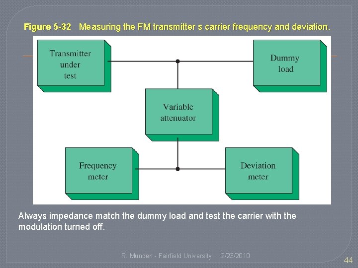
Figure 5 -32 Measuring the FM transmitter s carrier frequency and deviation. Always impedance match the dummy load and test the carrier with the modulation turned off. R. Munden - Fairfield University 2/23/2010 44
5 -11 Troubleshooting with Multisim R. Munden - Fairfield University 2/23/2010 45
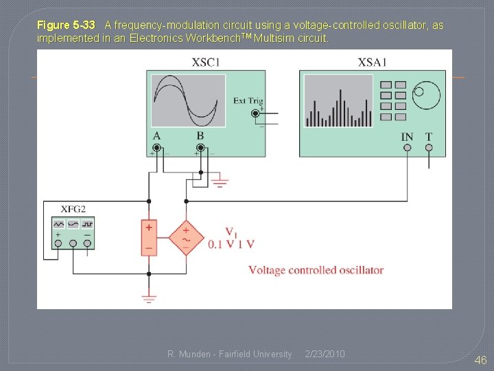
Figure 5 -33 A frequency-modulation circuit using a voltage-controlled oscillator, as implemented in an Electronics Workbench. TM Multisim circuit. R. Munden - Fairfield University 2/23/2010 46
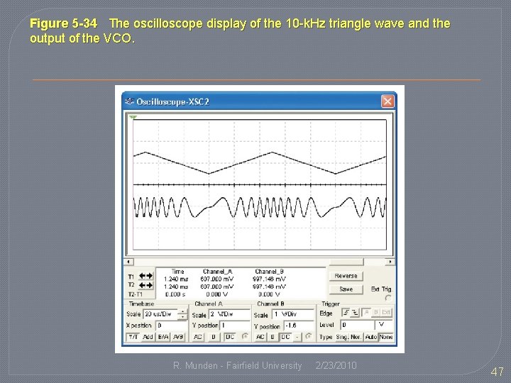
Figure 5 -34 The oscilloscope display of the 10 -k. Hz triangle wave and the output of the VCO. R. Munden - Fairfield University 2/23/2010 47
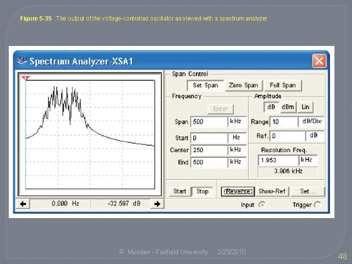
Figure 5 -35 The output of the voltage-controlled oscillator as viewed with a spectrum analyzer. R. Munden - Fairfield University 2/23/2010 48