CSCE 350 Algorithms and Data Structure Lecture 14

CSCE 350 Algorithms and Data Structure Lecture 14 Jianjun Hu Department of Computer Science and Engineering University of South Carolina 2009. 10.

Announcements Midterm 2 – Thursday Oct 29 in class As in Midterm 1, you will be allowed to bring in one single-side letter-size cheat sheet. For the good cheat sheets, we will give you bonus points – 5 points

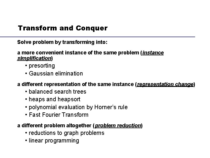
Transform and Conquer Solve problem by transforming into: a more convenient instance of the same problem (instance simplification) • presorting • Gaussian elimination a different representation of the same instance (representation change) • • balanced search trees heaps and heapsort polynomial evaluation by Horner’s rule Fast Fourier Transform a different problem altogether (problem reduction) • reductions to graph problems • linear programming

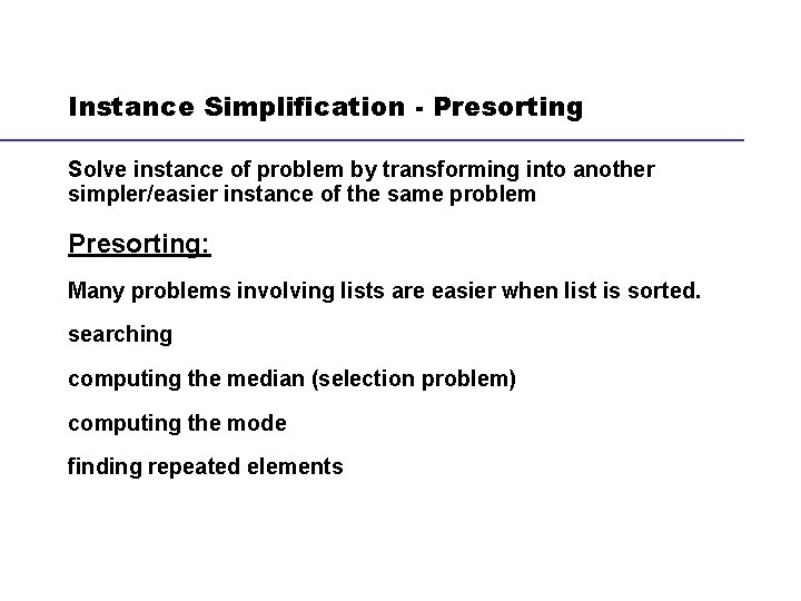
Instance Simplification - Presorting Solve instance of problem by transforming into another simpler/easier instance of the same problem Presorting: Many problems involving lists are easier when list is sorted. searching computing the median (selection problem) computing the mode finding repeated elements

Selection Problem Find the kth smallest element in A[1], …A[n]. Special cases: • minimum: k = 1 • maximum: k = n • median: k = n/2 Presorting-based algorithm • sort list • return A[k] Partition-based algorithm (Variable decrease & conquer): • pivot/split at A[s] using partitioning algorithm from quicksort • if s=k return A[s] • else if s<k repeat with sublist A[s+1], …A[n]. • else if s>k repeat with sublist A[1], …A[s-1].

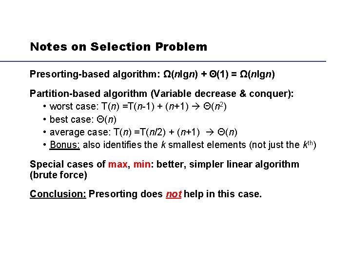
Notes on Selection Problem Presorting-based algorithm: Ω(nlgn) + Θ(1) = Ω(nlgn) Partition-based algorithm (Variable decrease & conquer): • worst case: T(n) =T(n-1) + (n+1) Θ(n 2) • best case: Θ(n) • average case: T(n) =T(n/2) + (n+1) Θ(n) • Bonus: also identifies the k smallest elements (not just the kth) Special cases of max, min: better, simpler linear algorithm (brute force) Conclusion: Presorting does not help in this case.

Finding Repeated Elements Presorting-based algorithm: • use mergesort (optimal): Θ(nlgn) • scan array to find repeated adjacent elements: Θ(n) Brute force algorithm: Θ(n 2) Conclusion: Presorting yields significant improvement Θ(nlgn)

Computing A Mode A mode is a value that occurs most often in a given list of numbers For example: the mode of [5, 1, 5, 7, 6, 5, 7] is 5 Brute-force technique: construct a list to record the frequency of each distinct element • In each iteration, the i-th element is compared to the stored distinct elements. If a matching is found, its frequency is incremented by 1. Otherwise, current element is added to the list as a distinct element • Worst case complexity Θ(n 2), when all the given n elements are distinct

Computing A Mode With Presorting Algorithm

Complexity of Presort. Mode() The dominating part is on the sorting Θ(nlgn) The complexity of the outer while loop is linear since each element will be visited once for comparison Therefore, the complexity of presort. Mode is Θ(nlgn) This is much more efficient than the brute-force algorithm that needs Θ(n 2)

Searching Problem Brute-force search: worst case Θ(n). Presorted search T(n)=Tsort(n)+ Tsearch(n) = Θ(n log n)+ Θ(log n) = Θ(n log n) Binary search Therefore, the presorted search is inferior to the brute-force search However, if we are going to repeat the searching in the same list many times, presorted search may be more efficient because the sorting need not be repeated

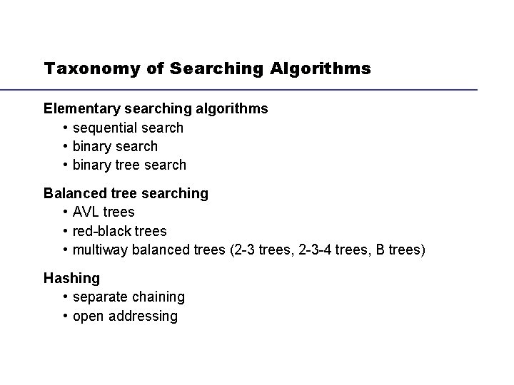
Taxonomy of Searching Algorithms Elementary searching algorithms • sequential search • binary tree search Balanced tree searching • AVL trees • red-black trees • multiway balanced trees (2 -3 trees, 2 -3 -4 trees, B trees) Hashing • separate chaining • open addressing

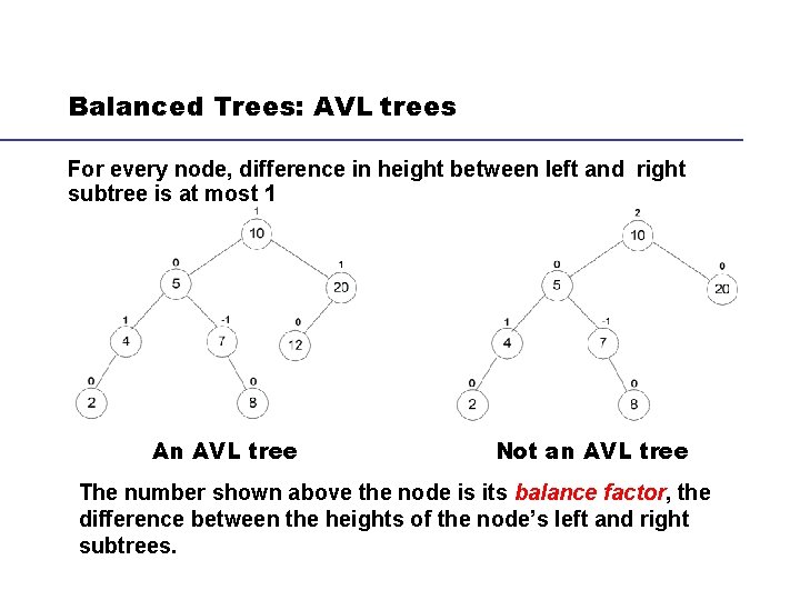
Balanced Trees: AVL trees For every node, difference in height between left and right subtree is at most 1 An AVL tree Not an AVL tree The number shown above the node is its balance factor, the difference between the heights of the node’s left and right subtrees.

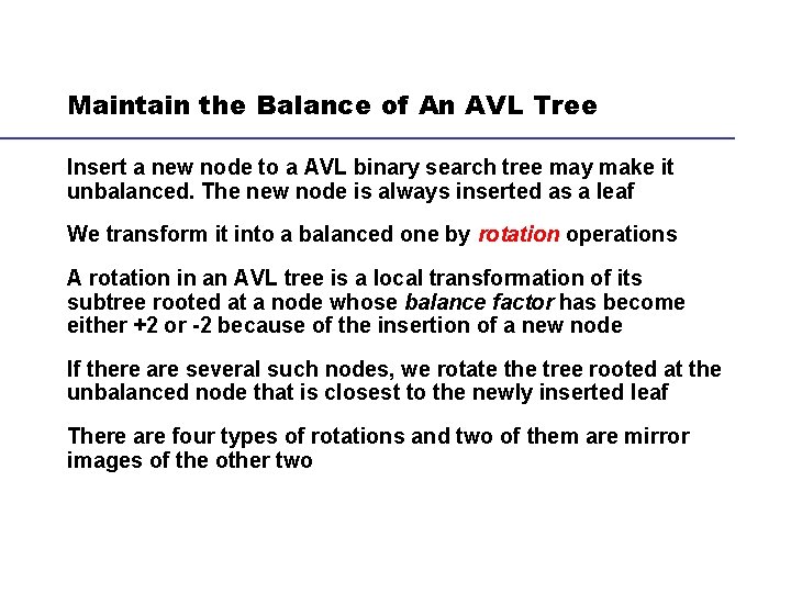
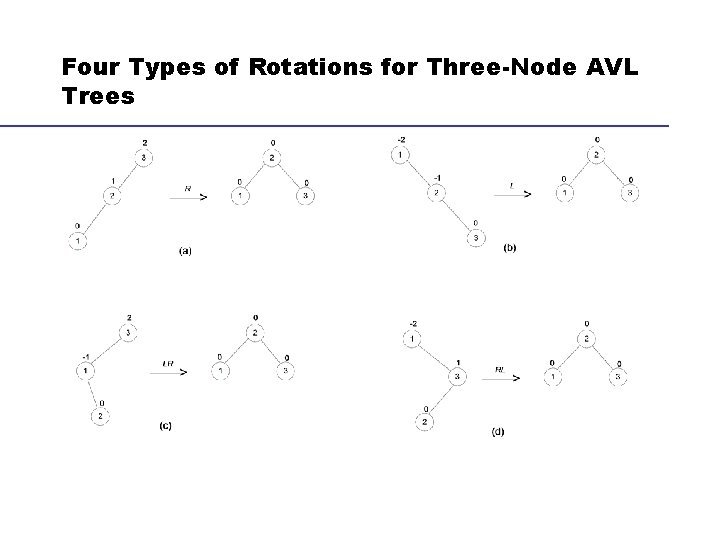
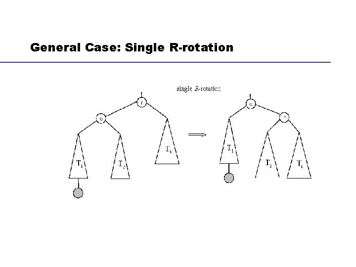
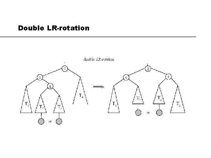
Maintain the Balance of An AVL Tree Insert a new node to a AVL binary search tree may make it unbalanced. The new node is always inserted as a leaf We transform it into a balanced one by rotation operations A rotation in an AVL tree is a local transformation of its subtree rooted at a node whose balance factor has become either +2 or -2 because of the insertion of a new node If there are several such nodes, we rotate the tree rooted at the unbalanced node that is closest to the newly inserted leaf There are four types of rotations and two of them are mirror images of the other two

Four Types of Rotations for Three-Node AVL Trees

General Case: Single R-rotation

Double LR-rotation

Notes on Rotations can be done in constant time (steps) Rotations not only guarantee that the resulting tree is balanced, but also should preserve the basic property of a binary search tree, i. e. , all the keys in the left subtree should be smaller than the root, the root should be smaller than all the keys in the right subtree. The height (h) of an AVL tree with n nodes is bounded by lg n ≤ h ≤ 1. 4404 lg (n + 2) - 1. 3277 average: 1. 01 lg n + 0. 1 for large n So the operations of searching and insertion in an AVL tree take Θ(logn) in the worst case

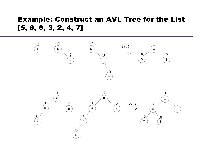
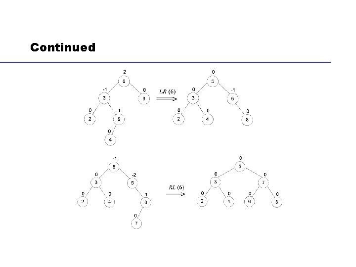
Example: Construct an AVL Tree for the List [5, 6, 8, 3, 2, 4, 7]

Continued

Other Trees Balance tree: Red-black trees (height of subtrees is allowed to differ by up to a factor of 2) and splay trees Allow more than one element in a node of a search tree: 2 -3 trees, 2 -3 -4 trees and B-trees. Read Section 6. 3 for more details.