Dynamic Causal Modelling Advanced Topics SPM Course f

Dynamic Causal Modelling Advanced Topics SPM Course (f. MRI), May 2015 Peter Zeidman Wellcome Trust Centre for Neuroimaging University College London

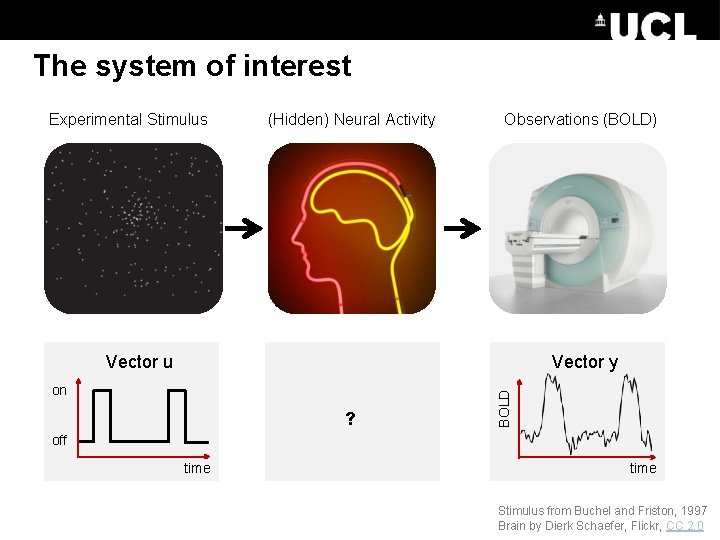
The system of interest Experimental Stimulus (Hidden) Neural Activity Observations (BOLD) Vector y on ? BOLD Vector u off time Stimulus from Buchel and Friston, 1997 Brain by Dierk Schaefer, Flickr, CC 2. 0

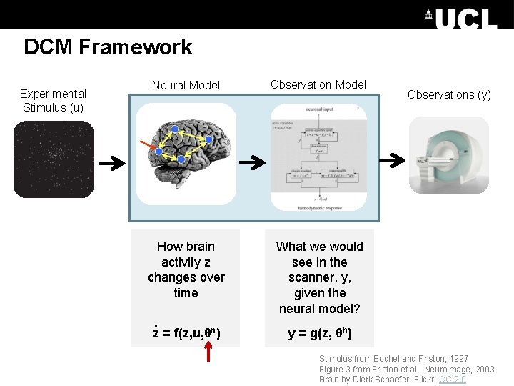
DCM Framework Experimental Stimulus (u) Neural Model Observation Model How brain activity z changes over time What we would see in the scanner, y, given the neural model? . z = f(z, u, θn) Observations (y) y = g(z, θh) Stimulus from Buchel and Friston, 1997 Figure 3 from Friston et al. , Neuroimage, 2003 Brain by Dierk Schaefer, Flickr, CC 2. 0

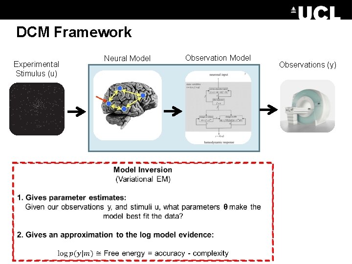
DCM Framework Experimental Stimulus (u) Neural Model Observations (y)

Contents • Creating models – Preparing data for DCM • Inference over models – Fixed Effects – Random Effects • Inference over parameters – Bayesian Model Averaging • Example • DCM Extensions

PREPARING DATA

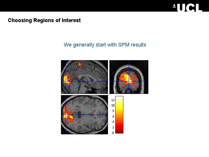
Choosing Regions of Interest We generally start with SPM results 12 10 8 6 4 2 0

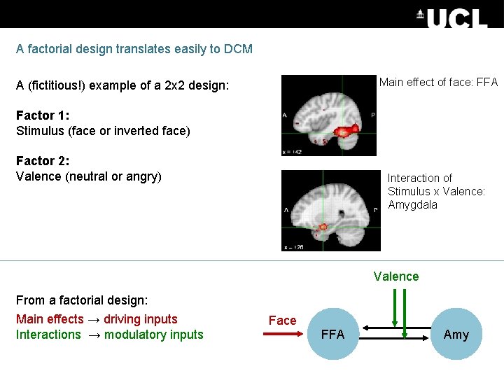
A factorial design translates easily to DCM Main effect of face: FFA A (fictitious!) example of a 2 x 2 design: Factor 1: Stimulus (face or inverted face) Factor 2: Valence (neutral or angry) Interaction of Stimulus x Valence: Amygdala Valence From a factorial design: Main effects → driving inputs Interactions → modulatory inputs Face FFA Amy

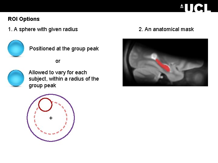
ROI Options 1. A sphere with given radius Positioned at the group peak or Allowed to vary for each subject, within a radius of the group peak + 2. An anatomical mask

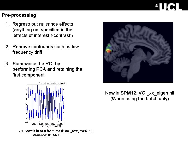
Pre-processing 1. Regress out nuisance effects (anything not specified in the ‘effects of interest f-contrast’) 2. Remove confounds such as low frequency drift 3. Summarise the ROI by performing PCA and retaining the first component 1 st eigenvariate: test 3 New in SPM 12: VOI_xx_eigen. nii (When using the batch only) 2 1 0 -1 -2 -3 -4 200 400 600 800 1000 time {seconds} 230 voxels in VOI from mask VOI_test_mask. nii Variance: 81. 66%

Interim Summary: Preparing Data • DCM helps us to explain the coupling between regions showing an experimental effect • We can choose our Regions of Interest (ROIs) from any series of contrasts in our GLM • We use Principle Components Analysis (PCA) to summarise the voxels in each ROI as a single timeseries

Contents • Creating models – Preparing data for DCM • Inference over models – Fixed Effects – Random Effects • Inference over parameters – Bayesian Model Averaging • Example • DCM Extensions

INFERENCE OVER MODELS

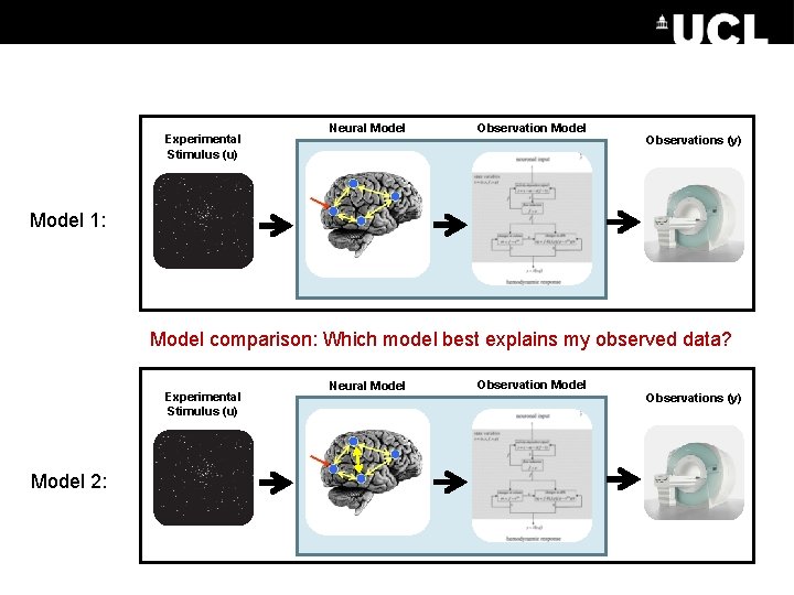
Experimental Stimulus (u) Neural Model Observations (y) Model 1: Model comparison: Which model best explains my observed data? Experimental Stimulus (u) Model 2: Neural Model Observations (y)

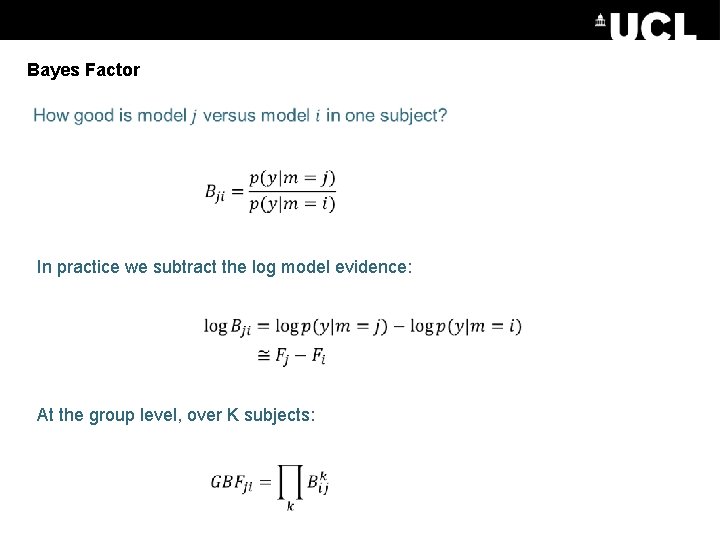
Bayes Factor In practice we subtract the log model evidence: At the group level, over K subjects:

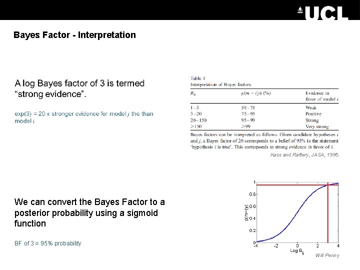
Bayes Factor - Interpretation Kass and Raftery, JASA, 1995. We can convert the Bayes Factor to a posterior probability using a sigmoid function BF of 3 = 95% probability Will Penny

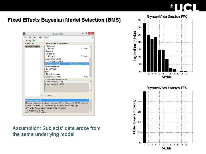
Fixed Effects Bayesian Model Selection (BMS) Assumption: Subjects’ data arose from the same underlying model

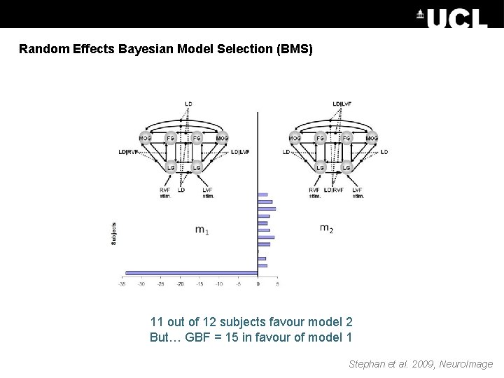
Random Effects Bayesian Model Selection (BMS) 11 out of 12 subjects favour model 2 But… GBF = 15 in favour of model 1 Stephan et al. 2009, Neuro. Image

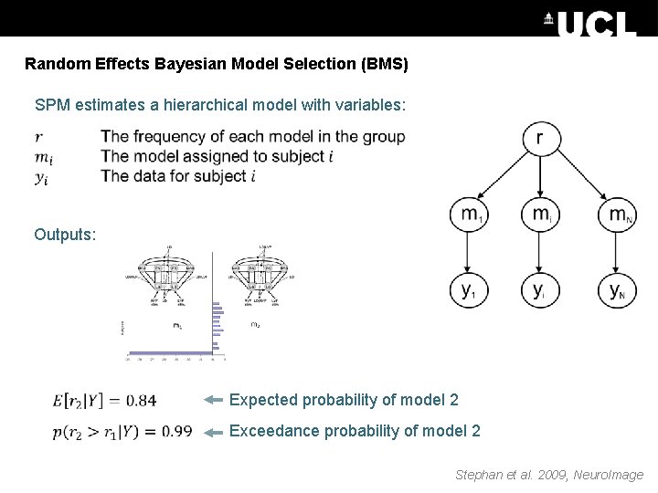
Random Effects Bayesian Model Selection (BMS) SPM estimates a hierarchical model with variables: Outputs: Expected probability of model 2 Exceedance probability of model 2 Stephan et al. 2009, Neuro. Image

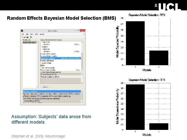
Random Effects Bayesian Model Selection (BMS) Assumption: Subjects’ data arose from different models Stephan et al. 2009, Neuro. Image

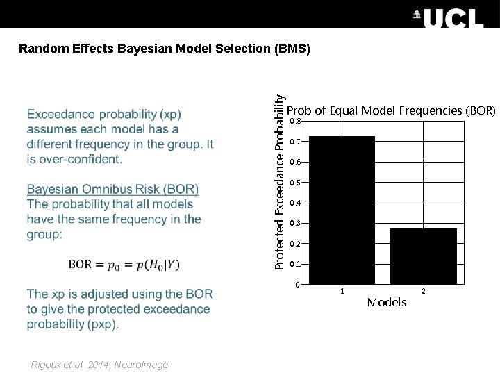
Protected Exceedance Probability Random Effects Bayesian Model Selection (BMS) Prob of Equal Model Frequencies (BOR) = 0. 8 0. 7 0. 6 0. 5 0. 4 0. 3 0. 2 0. 1 0 Rigoux et al. 2014, Neuro. Image 1 Models 2

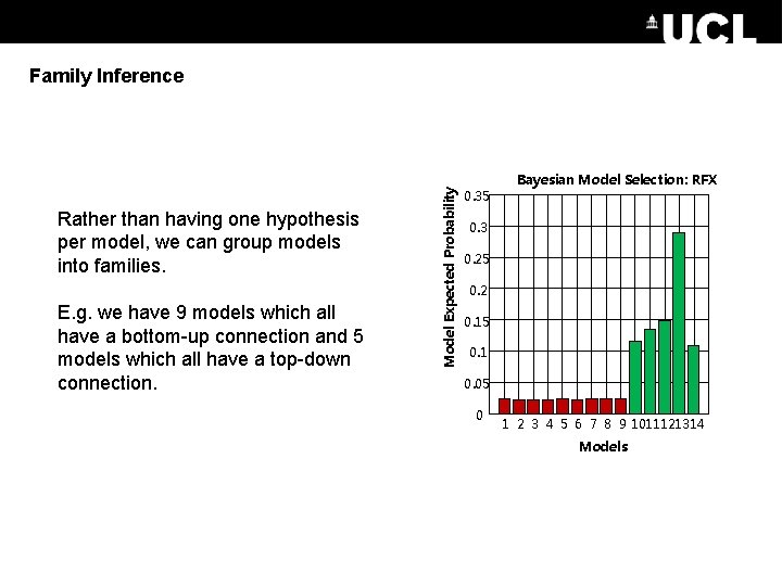
Rather than having one hypothesis per model, we can group models into families. E. g. we have 9 models which all have a bottom-up connection and 5 models which all have a top-down connection. Model Expected Probability Family Inference 0. 35 Bayesian Model Selection: RFX 0. 3 0. 25 0. 2 0. 15 0. 1 0. 05 0 1 2 3 4 5 6 7 8 9 1011121314 Models

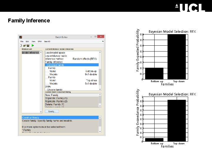
Family Expected Probability Family Inference 0. 8 Bayesian Model Selection: RFX 0. 7 0. 6 0. 5 0. 4 0. 3 0. 2 0. 1 0 Bottom-up Top-down Family Exceedance Probability Families 1 Bayesian Model Selection: RFX 0. 9 0. 8 0. 7 0. 6 0. 5 0. 4 0. 3 0. 2 0. 1 0 Bottom-up Top-down Families

Interim Summary: Inference over Models • We embody each of our hypotheses as a model or as a family of models. • We can compare models or families using a fixed effects analysis, only if we believe that all subjects have the same underlying model • Otherwise we use a random effects analysis and report the protected exceedance probability and the Bayesian Omnibus Risk.

Contents • Creating models – Preparing data for DCM • Inference over models – Fixed Effects – Random Effects • Inference over parameters – Bayesian Model Averaging • Example • DCM Extensions

INFERENCE OVER PARAMETERS

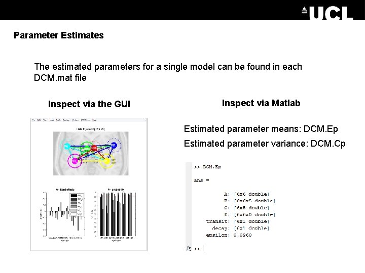
Parameter Estimates The estimated parameters for a single model can be found in each DCM. mat file Inspect via the GUI Inspect via Matlab Estimated parameter means: DCM. Ep Estimated parameter variance: DCM. Cp

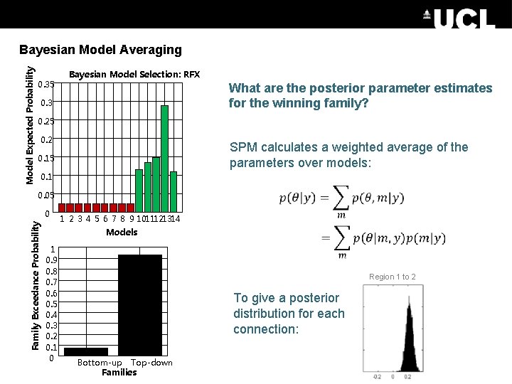
Model Expected Probability Bayesian Model Averaging 0. 35 Bayesian Model Selection: RFX What are the posterior parameter estimates for the winning family? 0. 3 0. 25 0. 2 SPM calculates a weighted average of the parameters over models: 0. 15 0. 1 0. 05 Family Exceedance Probability 0 1 2 3 4 5 6 7 8 9 1011121314 Models 1 0. 9 0. 8 0. 7 0. 6 0. 5 0. 4 0. 3 0. 2 0. 1 0 Region 1 to 2 To give a posterior distribution for each connection: Bottom-up Top-down Families

Contents • Creating models – Preparing data for DCM • Inference over models – Fixed Effects – Random Effects • Inference over parameters – Bayesian Model Averaging • Example • DCM Extensions

EXAMPLE

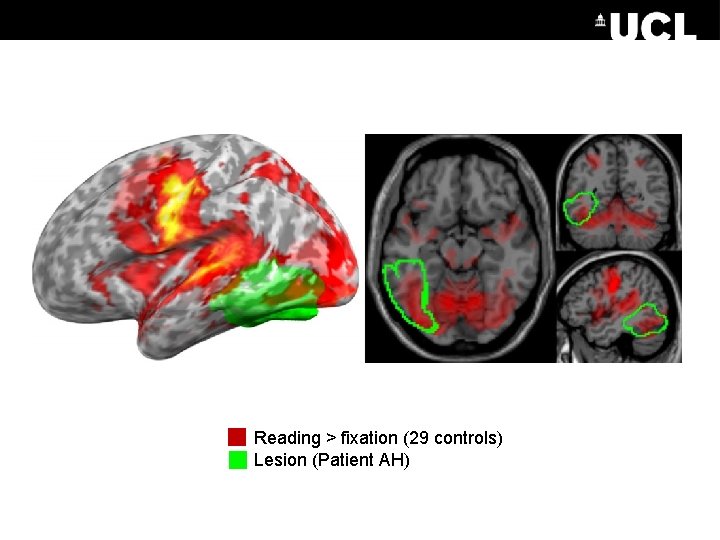
Reading > fixation (29 controls) Lesion (Patient AH)

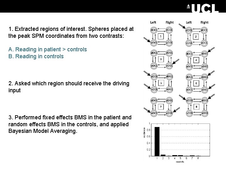
1. Extracted regions of interest. Spheres placed at the peak SPM coordinates from two contrasts: A. Reading in patient > controls B. Reading in controls 2. Asked which region should receive the driving input 3. Performed fixed effects BMS in the patient and random effects BMS in the controls, and applied Bayesian Model Averaging.

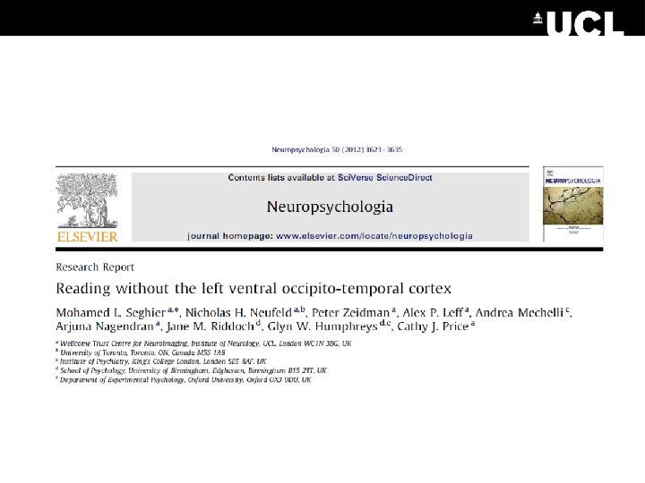
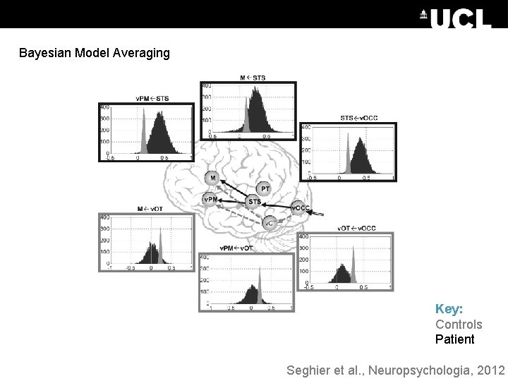
Bayesian Model Averaging Key: Controls Patient Seghier et al. , Neuropsychologia, 2012

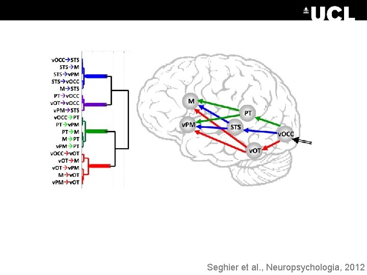
Seghier et al. , Neuropsychologia, 2012

Interim Summary: Example • When we don’t know how to model something, we can ‘ask the data’ using a model comparison • Bayesian Model Averaging (BMA) lets us compare connections across patients and controls • Posterior parameter estimates can be used as summary statistics for further analyses

DCM EXTENSIONS

DCM Framework Experimental Stimulus (u) Neural Model Observation Model How brain activity z changes over time What we would see in the scanner, y, given the neural model? . z = f(z, u, θn) Observations (y) y = g(z, θh) Stimulus from Buchel and Friston, 1997 Figure 3 from Friston et al. , Neuroimage, 2003 Brain by Dierk Schaefer, Flickr, CC 2. 0

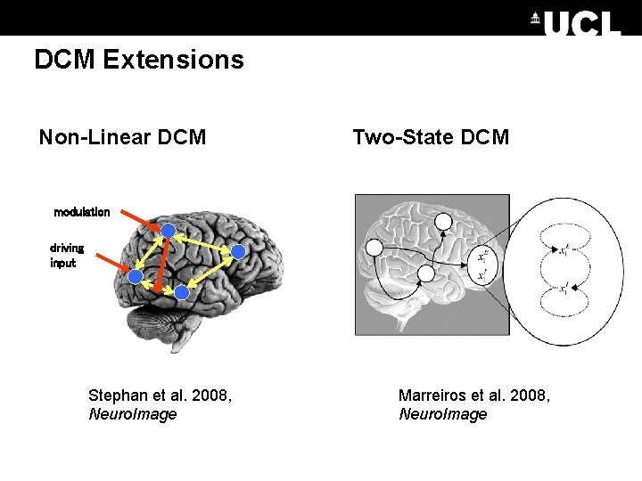
DCM Extensions Non-Linear DCM Two-State DCM modulation driving input Stephan et al. 2008, Neuro. Image Marreiros et al. 2008, Neuro. Image

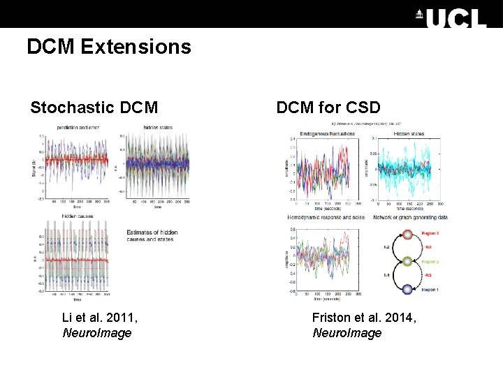
DCM Extensions Stochastic DCM Li et al. 2011, Neuro. Image DCM for CSD Friston et al. 2014, Neuro. Image

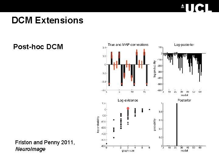
DCM Extensions Post-hoc DCM Friston and Penny 2011, Neuro. Image

Further Reading The original DCM paper Friston et al. 2003, Neuro. Image Descriptive / tutorial papers Role of General Systems Theory Stephan 2004, J Anatomy DCM: Ten simple rules for the clinician Kahan et al. 2013, Neuro. Image Ten Simple Rules for DCM Stephan et al. 2010, Neuro. Image DCM Extensions Two-state DCM Marreiros et al. 2008, Neuro. Image Non-linear DCM Stephan et al. 2008, Neuro. Image Stochastic DCM Li et al. 2011, Neuro. Image Friston et al. 2011, Neuro. Image Daunizeau et al. 2012, Front Comput Neurosci Post-hoc DCM Friston and Penny, 2011, Neuro. Image Rosa and Friston, 2012, J Neuro Methods A DCM for Resting State f. MRI Friston et al. , 2014, Neuro. Image

EXTRAS

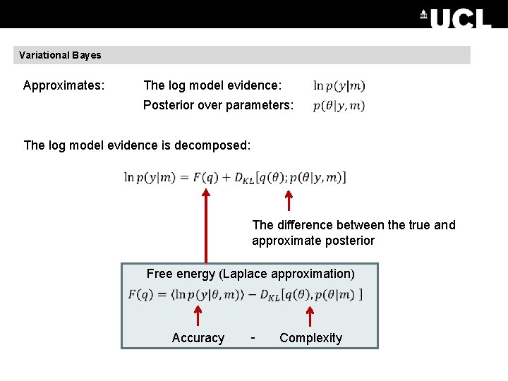
Variational Bayes Approximates: The log model evidence: Posterior over parameters: The log model evidence is decomposed: The difference between the true and approximate posterior Free energy (Laplace approximation) Accuracy - Complexity

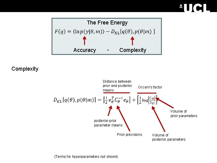
The Free Energy Accuracy - Complexity Distance between prior and posterior means Occam’s factor Volume of prior parameters posterior-prior parameter means Prior precisions (Terms for hyperparameters not shown) Volume of posterior parameters

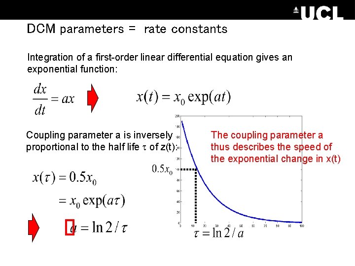
DCM parameters = rate constants Integration of a first-order linear differential equation gives an exponential function: Coupling parameter a is inversely proportional to the half life of z(t): The coupling parameter a thus describes the speed of the exponential change in x(t)

Practical Workshop

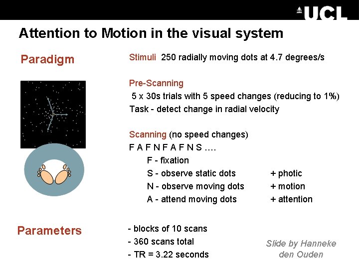
Attention to Motion in the visual system DCM – Attention. Stimuli 250 radially moving dots at 4. 7 degrees/s to Motion Paradigm Pre-Scanning 5 x 30 s trials with 5 speed changes (reducing to 1%) Task - detect change in radial velocity Scanning (no speed changes) F A F N S …. F - fixation S - observe static dots N - observe moving dots A - attend moving dots Parameters - blocks of 10 scans - 360 scans total - TR = 3. 22 seconds + photic + motion + attention Slide by Hanneke den Ouden

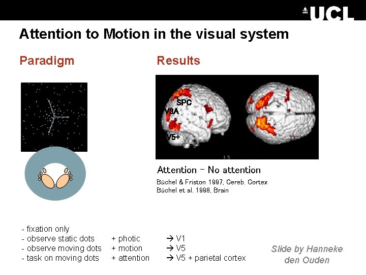
Attention to Motion in the visual system Paradigm Results SPC V 3 A V 5+ Attention – No attention Büchel & Friston 1997, Cereb. Cortex Büchel et al. 1998, Brain - fixation only - observe static dots - observe moving dots - task on moving dots + photic + motion + attention V 1 V 5 + parietal cortex Slide by Hanneke den Ouden

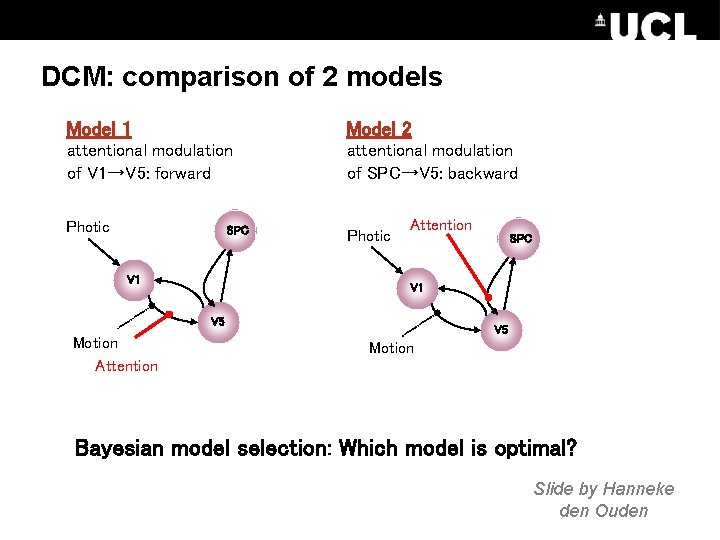
DCM: comparison of 2 models Model 1 Model 2 attentional modulation of V 1→V 5: forward attentional modulation of SPC→V 5: backward Photic SPC V 1 Photic Attention V 1 V 5 Motion Attention SPC V 5 Motion Bayesian model selection: Which model is optimal? Slide by Hanneke den Ouden

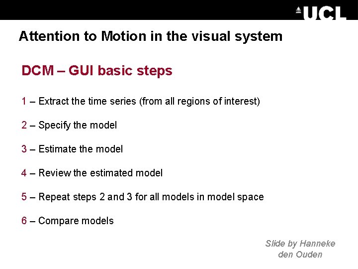
Attention to Motion in the visual system DCM – GUI basic steps 1 – Extract the time series (from all regions of interest) 2 – Specify the model 3 – Estimate the model 4 – Review the estimated model 5 – Repeat steps 2 and 3 for all models in model space 6 – Compare models Slide by Hanneke den Ouden