Dynamic Causal Modelling Introduction SPM Course f MRI

Dynamic Causal Modelling Introduction SPM Course (f. MRI), October 2015 Peter Zeidman Wellcome Trust Centre for Neuroimaging University College London

Dynamic Causal Modelling is a framework for creating, estimating and comparing generative models of neuroimaging timeseries We use these models to investigate effective connectivity of neuronal populations

Contents • Overview of DCM – Effective connectivity, DCM framework, generative models • Model specification – Neural model, haemodynamic model • Model estimation – Model inversion, parameter inference • Example

Contents • Overview of DCM – Effective connectivity, DCM framework, generative models • Model specification – Neural model, haemodynamic model • Model estimation – Model inversion, parameter inference • Example

The system of interest Experimental Stimulus (Hidden) Neural Activity Observations (BOLD) Vector y on ? BOLD Vector u off time Stimulus from Buchel and Friston, 1997 Brain by Dierk Schaefer, Flickr, CC 2. 0

Connectivity • Structural Connectivity Physical connections of the brain • Functional Connectivity Dependencies between BOLD observations • Effectivity Connectivity Causal relationships between brain regions "Connectome" by jgmarcelino. CC 2. 0 via Wikimedia Commons Figure 1, Hong et al. 2013 PLOS ONE. KE Stefan, SPM Course 2011

DCM Framework Experimental Stimulus (u) Neural Model Observation Model How brain activity z changes over time What we would see in the scanner, y, given the neural model? . z = f(z, u, θn) Observations (y) y = g(z, θh) Stimulus from Buchel and Friston, 1997 Figure 3 from Friston et al. , Neuroimage, 2003 Brain by Dierk Schaefer, Flickr, CC 2. 0

DCM Framework Experimental Stimulus (u) Neural Model Observations (y) Generative model p(u, y) Stimulus from Buchel and Friston, 1997 Figure 3 from Friston et al. , Neuroimage, 2003 Brain by Dierk Schaefer, Flickr, CC 2. 0

DCM Framework Experimental Stimulus (u) Neural Model Observations (y)

DCM Framework Experimental Stimulus (u) Neural Model Observations (y) Model 1: Model comparison: Which model best explains my observed data? Experimental Stimulus (u) Model 2: Neural Model Observations (y)

DCM Framework 1. We embody each of our hypotheses in a generative model. The generative model separates neural activity from haemodynamics 2. We perform model estimation (inversion) This identifies parameters θ = {θn, θh} which make the model best fit the data and the free energy (log model evidence) 3. We inspect the estimated parameters and / or we compare models to see which best explains the data.

Contents • Overview of DCM – Effective connectivity, DCM framework, generative models • Model specification – Neural model, haemodynamic model • Model estimation – Model inversion, parameter inference • Example

The Neural Model “How does brain activity, z, change over time? ” u 1 z 1 V 1 a c z 1 Driving input u 1 z 2 Inhibitory self-connection (Hz). Rate constant: controls rate of decay in region 1. More negative = faster decay.

The Neural Model “How does brain activity, z, change over time? ” Change of activity in V 1: z 2 V 5 a 22 a 21 Change of activity in V 5: z 1 V 1 c 11 Self decay V 1 input Driving input u 1 a 11

The Neural Model “How does brain activity, z, change over time? ” z 2 a 21 Columns are outgoing connections Rows are incoming connections z 1 V 5 V 1 c 11 Driving input u 1 a 11

The Neural Model “How does brain activity, z, change over time? ” z 2 u 1 z 2 V 5 a 22 a 21 z 1 V 1 c 11 Driving input u 1 a 11

The Neural Model “How does brain activity, z, change over time? ” z 2 u 1 b 21 u 2 Attention u 2 z 1 V 5 a 21 V 1 c 11 z 2 Could model be used to model a main effect and interaction a 22 Driving input u 1 a 11

The Neural Model “How does brain activity, z, change over time? ” Change of activity in V 1: z 2 b 21 Attention u 2 Change of activity in V 5: z 1 V 5 a 22 a 21 V 1 a 11 c 11 Self decay V 1 input Modulatory input Driving input u 1

The Neural Model V 5 z 2 b 21 “How does brain activity, z, change over time? ” a 21 Attention u 2 V 1 z 1 For m inputs: a 22 a 11 c 11 Driving input u 1 A: Structure B: Modulatory Input C: Driving Input Change in activity per region External input 2 (attention) Current activity per region All external input

DCM Framework Experimental Stimulus (u) Neural Model Observation Model How brain activity z changes over time What we would see in the scanner, y, given the neural model? . z = f(z, u, θn) Observations (y) y = g(z, θh) Stimulus from Buchel and Friston, 1997 Figure 3 from Friston et al. , Neuroimage, 2003 Brain by Dierk Schaefer, Flickr, CC 2. 0

The Haemodynamic Model

Contents • Overview of DCM – Effective connectivity, DCM framework, generative models • Model specification – Neural model, haemodynamic model • Model estimation – Model inversion, parameter inference • Example

DCM Framework Experimental Stimulus (u) Neural Model Observation Model How brain activity z changes over time What we would see in the scanner, y, given the neural model? . z = f(z, u, θn) Observations (y) y = g(z, θh) Stimulus from Buchel and Friston, 1997 Figure 3 from Friston et al. , Neuroimage, 2003 Brain by Dierk Schaefer, Flickr, CC 2. 0

Bayesian Models new data prior knowledge posterior likelihood ∙ prior parameter estimates

Priors Prior means stored in DCM. M. p. E, covariance in DCM. M. p. C Prior on between-region coupling N(0, 1/64) -1 -0. 5 0 0. 5 Connection strength (Hz) 1

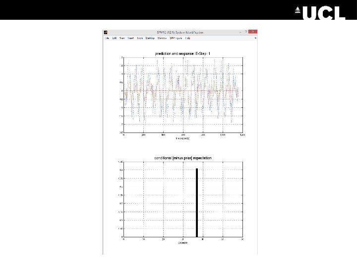
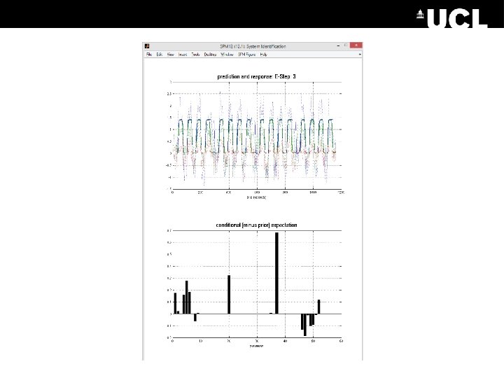
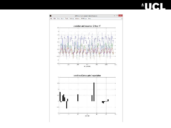
Model Estimation Posterior mean stored in DCM. Ep Posterior variance stored in DCM. Vp. Noise precision stored in DCM. Ce Free energy stored in DCM. F

Bayesian Model Reduction Model 1 Model 2 Model 3 Option 1: Individually fit each model to the data (then inspect or compare) Option 2: Fit only the full model (model 1) then use ‘post-hoc model reduction’ (Bayesian Model Reduction) to estimate the others

Contents • Overview of DCM – Effective connectivity, DCM framework, generative models • Model specification – Neural model, haemodynamic model • Model estimation – Model inversion, parameter inference • Example

PREPARING DATA

Choosing Regions of Interest We generally start with SPM results 12 10 8 6 4 2 0

ROI Options 1. A sphere with given radius Positioned at the group peak or Allowed to vary for each subject, within a radius of the group peak + 2. An anatomical mask

Pre-processing 1. Regress out nuisance effects (anything not specified in the ‘effects of interest f-contrast’) 2. Remove confounds such as low frequency drift 3. Summarise the ROI by performing PCA and retaining the first component 1 st eigenvariate: test 3 New in SPM 12: VOI_xx_eigen. nii (When using the batch only) 2 1 0 -1 -2 -3 -4 200 400 600 800 1000 time {seconds} 230 voxels in VOI from mask VOI_test_mask. nii Variance: 81. 66%

EXAMPLE

Reading > fixation (29 controls) Lesion (Patient AH)

1. Extracted regions of interest. Spheres placed at the peak SPM coordinates from two contrasts: A. Reading in patient > controls B. Reading in controls 2. Asked which region should receive the driving input

Bayesian Model Averaging Key: Controls Patient Seghier et al. , Neuropsychologia, 2012

Seghier et al. , Neuropsychologia, 2012

TROUBLESHOOTING

spm_dcm_fmri_check(DCM) spm_dcm_explore (DCM) From Jean Daunizeau’s website

Further Reading The original DCM paper Friston et al. 2003, Neuro. Image Descriptive / tutorial papers Role of General Systems Theory Stephan 2004, J Anatomy DCM: Ten simple rules for the clinician Kahan et al. 2013, Neuro. Image Ten Simple Rules for DCM Stephan et al. 2010, Neuro. Image DCM Extensions Two-state DCM Marreiros et al. 2008, Neuro. Image Non-linear DCM Stephan et al. 2008, Neuro. Image Stochastic DCM Li et al. 2011, Neuro. Image Friston et al. 2011, Neuro. Image Daunizeau et al. 2012, Front Comput Neurosci Post-hoc DCM Friston and Penny, 2011, Neuro. Image Rosa and Friston, 2012, J Neuro Methods A DCM for Resting State f. MRI Friston et al. , 2014, Neuro. Image

EXTRAS

Variational Bayes Approximates: The log model evidence: Posterior over parameters: The log model evidence is decomposed: The difference between the true and approximate posterior Free energy (Laplace approximation) Accuracy - Complexity

The Free Energy Accuracy - Complexity Distance between prior and posterior means Occam’s factor Volume of prior parameters posterior-prior parameter means Prior precisions (Terms for hyperparameters not shown) Volume of posterior parameters

DCM parameters = rate constants Integration of a first-order linear differential equation gives an exponential function: Coupling parameter a is inversely proportional to the half life of x(t): The coupling parameter ‘a’ thus describes the speed of the exponential change in x(t)

A factorial design translates easily to DCM A (fictitious!) example of a 2 x 2 design: Main effect of face: FFA Factor 1: Stimulus (face or inverted face) Factor 2: Valence (neutral or angry) Interaction of Stimulus x Valence: Amygdala Valence From a factorial design: Main effects → driving inputs Face FF Interactions → modulatory inputs A A my