Duarte Wakin Compressed Sensing meets Information Theory Sarvotham

Duarte Wakin Compressed Sensing meets Information Theory Sarvotham Baraniuk Dror Baron drorb@ee. technion. ac. il www. ee. technion. ac. il/people/drorb Guo Shamai

Technology Breakthroughs • Sensing, Computation, Communication – fast, readily available, cheap • Progress in individual disciplines (computing, networks, comm, DSP, …)

The Data Deluge

The Data Deluge • Challenges: – Exponentially increasing amounts of data § myriad different modalities (audio, image, video, financial, seismic, weather …) § global scale acquisition – Analysis/processing hampered by slowing Moore’s law § finding “needle in haystack” – Energy consumption • Opportunities (today)

From Sampling to Compressed Sensing

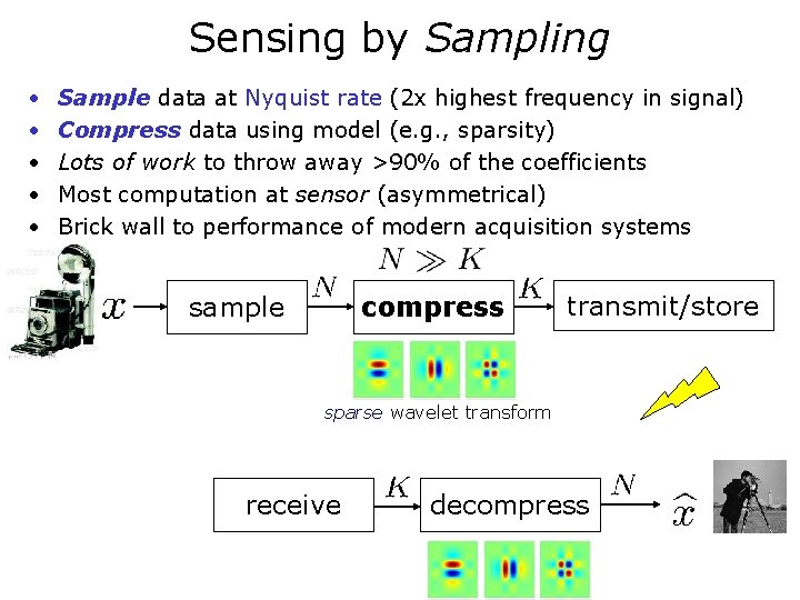
Sensing by Sampling • • • Sample data at Nyquist rate (2 x highest frequency in signal) Compress data using model (e. g. , sparsity) Lots of work to throw away >90% of the coefficients Most computation at sensor (asymmetrical) Brick wall to performance of modern acquisition systems sample compress transmit/store sparse wavelet transform receive decompress

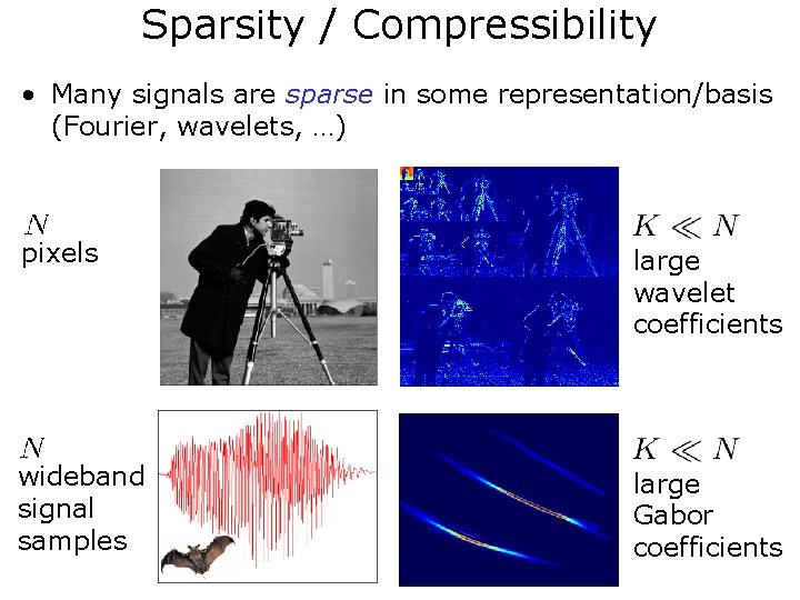
Sparsity / Compressibility • Many signals are sparse in some representation/basis (Fourier, wavelets, …) pixels large wavelet coefficients wideband signal samples large Gabor coefficients

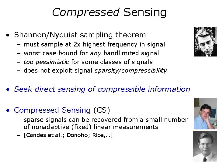
Compressed Sensing • Shannon/Nyquist sampling theorem – – must sample at 2 x highest frequency in signal worst case bound for any bandlimited signal too pessimistic for some classes of signals does not exploit signal sparsity/compressibility • Seek direct sensing of compressible information • Compressed Sensing (CS) – sparse signals can be recovered from a small number of nonadaptive (fixed) linear measurements – [Candes et al. ; Donoho; Rice, …]

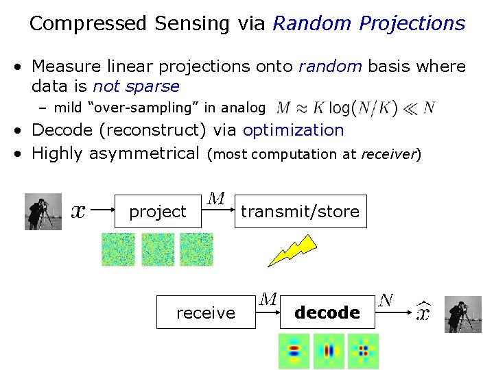
Compressed Sensing via Random Projections • Measure linear projections onto random basis where data is not sparse – mild “over-sampling” in analog • Decode (reconstruct) via optimization • Highly asymmetrical (most computation at receiver) project receive transmit/store decode

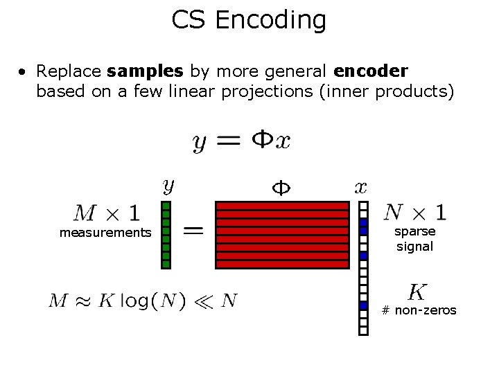
CS Encoding • Replace samples by more general encoder based on a few linear projections (inner products) measurements sparse signal # non-zeros

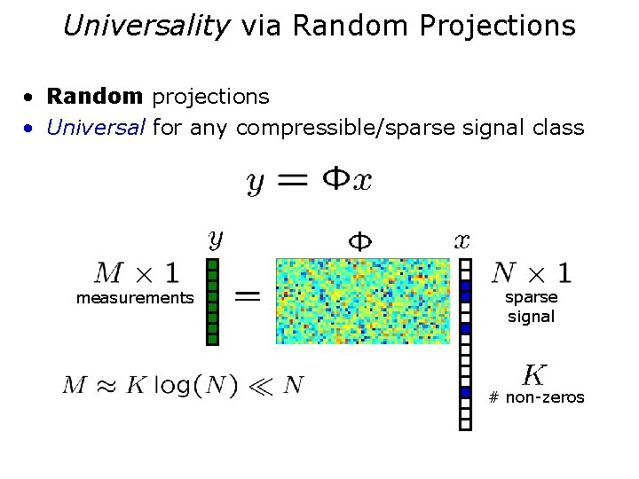
Universality via Random Projections • Random projections • Universal for any compressible/sparse signal class measurements sparse signal # non-zeros

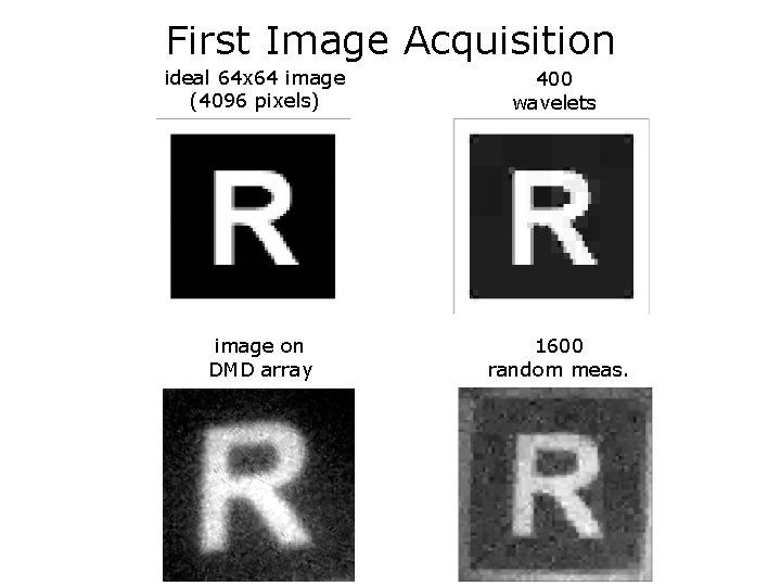
Optical Computation of Random Projections [Rice DSP 2006] • CS measurements directly in analog • Single photodiode

First Image Acquisition ideal 64 x 64 image (4096 pixels) 400 wavelets image on DMD array 1600 random meas.

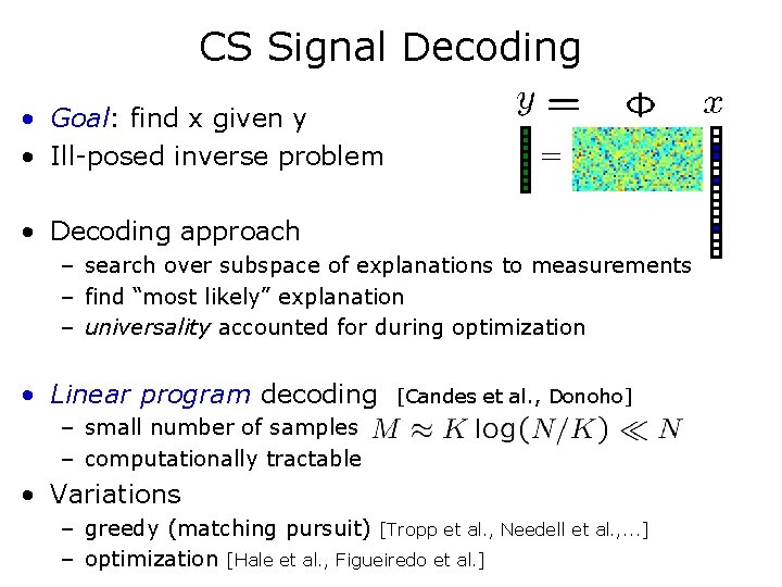
CS Signal Decoding • Goal: find x given y • Ill-posed inverse problem • Decoding approach – search over subspace of explanations to measurements – find “most likely” explanation – universality accounted for during optimization • Linear program decoding [Candes et al. , Donoho] – small number of samples – computationally tractable • Variations – greedy (matching pursuit) [Tropp et al. , Needell et al. , . . . ] – optimization [Hale et al. , Figueiredo et al. ]

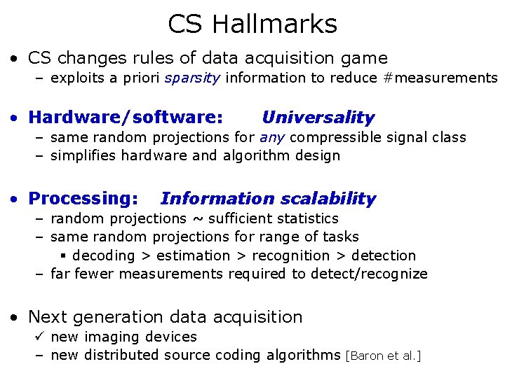
CS Hallmarks • CS changes rules of data acquisition game – exploits a priori sparsity information to reduce #measurements • Hardware/software: Universality – same random projections for any compressible signal class – simplifies hardware and algorithm design • Processing: Information scalability – random projections ~ sufficient statistics – same random projections for range of tasks § decoding > estimation > recognition > detection – far fewer measurements required to detect/recognize • Next generation data acquisition ü new imaging devices – new distributed source coding algorithms [Baron et al. ]

CS meets Information Theoretic Bounds [Sarvotham, Baron, & Baraniuk 2006] [Guo, Baron, & Shamai 2009]

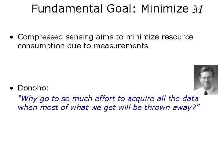
Fundamental Goal: Minimize • Compressed sensing aims to minimize resource consumption due to measurements • Donoho: “Why go to so much effort to acquire all the data when most of what we get will be thrown away? ”

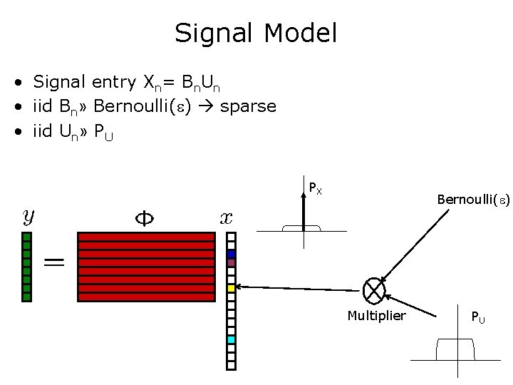
Signal Model • Signal entry Xn= Bn. Un • iid Bn» Bernoulli( ) sparse • iid Un» PU PX Bernoulli( ) Multiplier PU

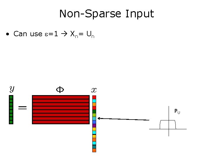
Non-Sparse Input • Can use =1 Xn= Un PU

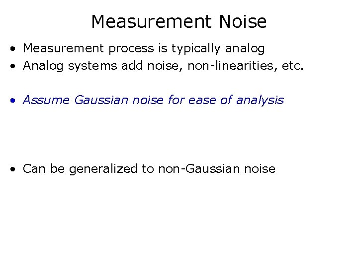
Measurement Noise • Measurement process is typically analog • Analog systems add noise, non-linearities, etc. • Assume Gaussian noise for ease of analysis • Can be generalized to non-Gaussian noise

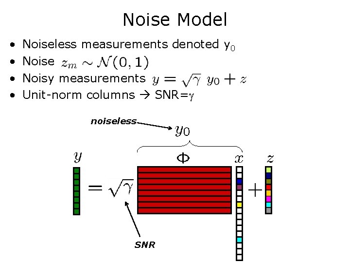
Noise Model • • Noiseless measurements denoted y 0 Noise Noisy measurements Unit-norm columns SNR= noiseless SNR

CS Analog to Communication System [Sarvotham, Baron, & Baraniuk 2006] • Model process source encoder channel encoder CS measurement as measurement channel decoder source decoder CS decoding • Measurements provide information!

Single-Letter Bounds • Theorem: [Sarvotham, Baron, & Baraniuk 2006] For sparse signal with rate-distortion function R(D), lower bound on measurement rate s. t. SNR and distortion D • Numerous single-letter bounds – – – – [Aeron, Zhao, & Saligrama] [Akcakaya & Tarokh] [Rangan, Fletcher, & Goyal] [Gastpar & Reeves] [Wang, Wainwright, & Ramchandran] [Tune, Bhaskaran, & Hanly] …

Goal: Precise Single-letter Characterization of Optimal CS [Guo, Baron, & Shamai 2009]

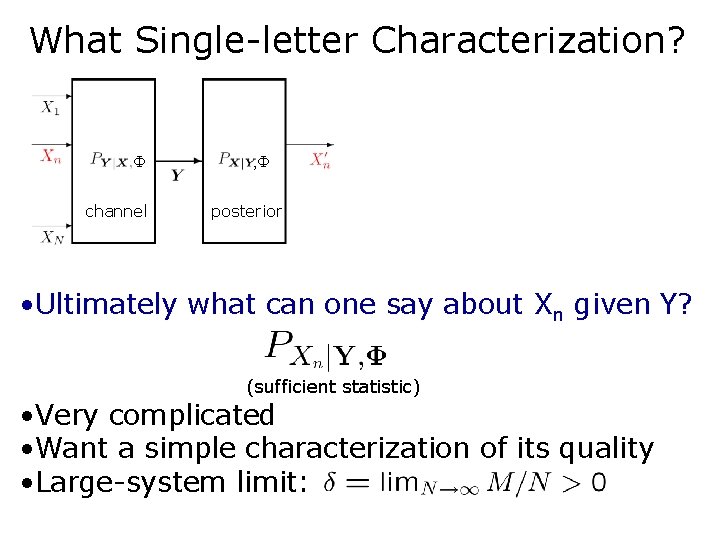
What Single-letter Characterization? channel , posterior • Ultimately what can one say about Xn given Y? (sufficient statistic) • Very complicated • Want a simple characterization of its quality • Large-system limit:

Main Result: Single-letter Characterization [Guo, Baron, & Shamai 2009] channel , • Result 1: Conditioned on Xn=xn, the observations (Y, ) are statistically equivalent to posterior degradation easy to compute… • Estimation quality from (Y, ) just as good as noisier scalar observation

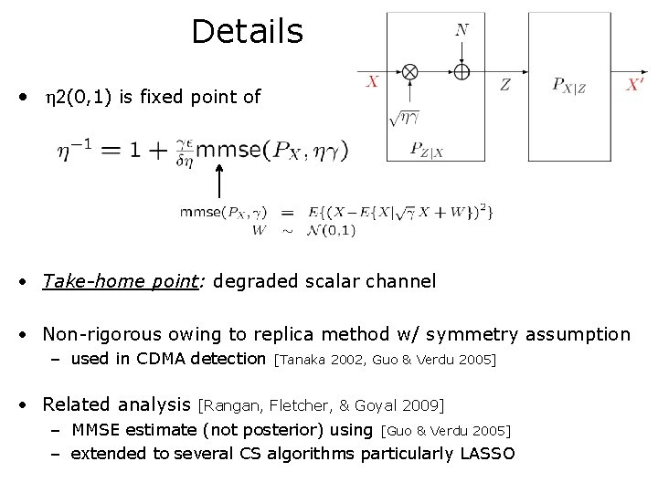
Details • 2(0, 1) is fixed point of • Take-home point: degraded scalar channel • Non-rigorous owing to replica method w/ symmetry assumption – used in CDMA detection • Related analysis [Tanaka 2002, Guo & Verdu 2005] [Rangan, Fletcher, & Goyal 2009] – MMSE estimate (not posterior) using [Guo & Verdu 2005] – extended to several CS algorithms particularly LASSO

Decoupling

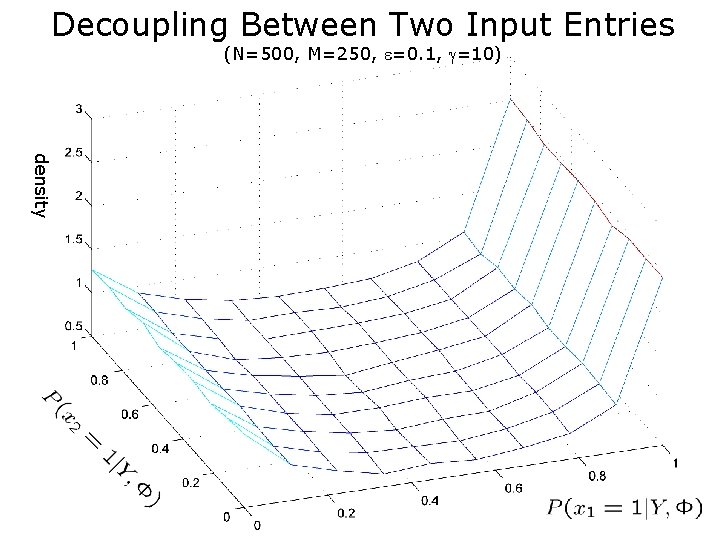
Decoupling Result [Guo, Baron, & Shamai 2009] • Result 2: Large system limit; any arbitrary (constant) L input elements decouple: • Take-home point: individual posteriors statistically independent

Sparse Measurement Matrices

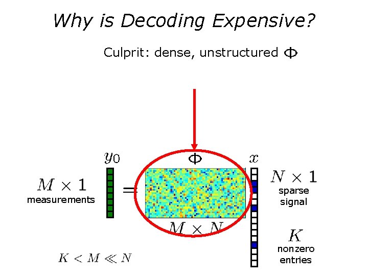
Why is Decoding Expensive? Culprit: dense, unstructured measurements sparse signal nonzero entries

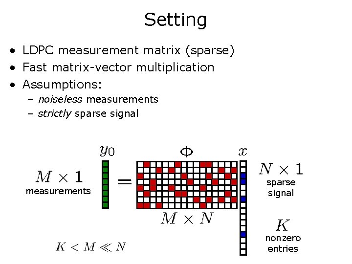
Sparse Measurement Matrices [Baron, Sarvotham, & Baraniuk 2009] • • LDPC measurement matrix (sparse) Mostly zeros in ; nonzeros » P Each row contains ¼Nq randomly placed nonzeros Fast matrix-vector multiplication ð fast encoding / decoding sparse matrix

CS Decoding Using BP [Baron, Sarvotham, & Baraniuk 2009] • Measurement matrix represented by graph • Estimate real-valued input iteratively • Implemented via nonparametric BP [Bickson, Sommer, …] signal x measurements y

Identical Single-letter Characterization w/BP [Guo, Baron, & Shamai 2009] • Result 3: Conditioned on Xn=xn, the observations (Y, ) are statistically equivalent to identical degradation • Sparse matrices just as good • Result 4: BP is asymptotically optimal!

Decoupling Between Two Input Entries (N=500, M=250, =0. 1, =10) density

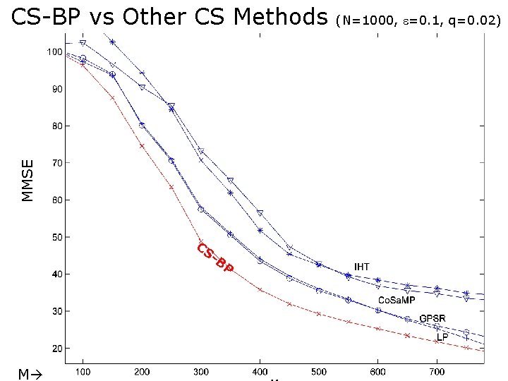
MMSE CS-BP vs Other CS Methods CS - BP M (N=1000, =0. 1, q=0. 02)

Runtime [seconds] CS-BP is O(Nlog 2(N)) N (M=0. 4 N, =0. 1, =100, q=0. 04)

Fast CS Decoding [Sarvotham, Baron, & Baraniuk 2006]

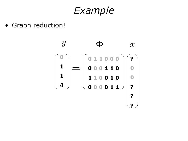
Setting • LDPC measurement matrix (sparse) • Fast matrix-vector multiplication • Assumptions: – noiseless measurements – strictly sparse signal measurements sparse signal nonzero entries

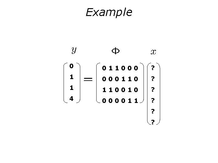
Example 0 011000 ? 1 000110 ? 1 110010 ? 4 000011 ? ? ?

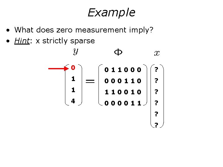
Example • What does zero measurement imply? • Hint: x strictly sparse 0 011000 ? 1 000110 ? 1 110010 ? 4 000011 ? ? ?

Example • Graph reduction! 0 011000 ? 1 000110 0 1 110010 0 4 000011 ? ? ?

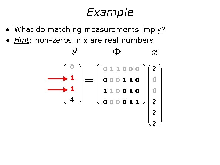
Example • What do matching measurements imply? • Hint: non-zeros in x are real numbers 0 011000 ? 1 000110 0 1 110010 0 4 000011 ? ? ?

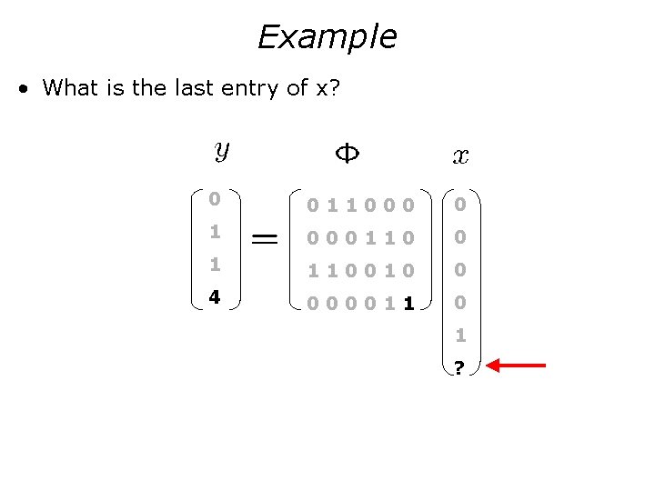
Example • What is the last entry of x? 0 011000 0 1 000110 0 1 110010 0 4 000011 0 1 ?

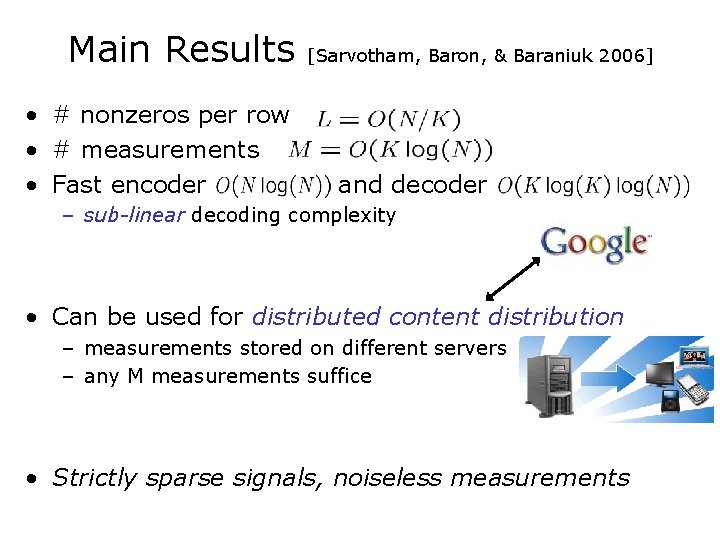
Main Results • # nonzeros per row • # measurements • Fast encoder [Sarvotham, Baron, & Baraniuk 2006] and decoder – sub-linear decoding complexity • Can be used for distributed content distribution – measurements stored on different servers – any M measurements suffice • Strictly sparse signals, noiseless measurements

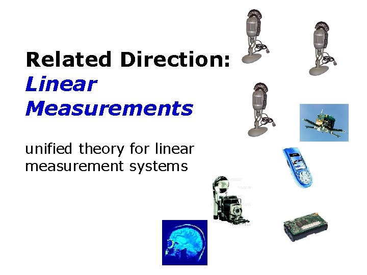
Related Direction: Linear Measurements unified theory for linear measurement systems

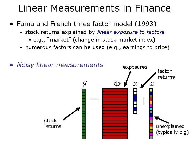
Linear Measurements in Finance • Fama and French three factor model (1993) – stock returns explained by linear exposure to factors § e. g. , “market” (change in stock market index) – numerous factors can be used (e. g. , earnings to price) • Noisy linear measurements stock returns exposures factor returns unexplained (typically big)

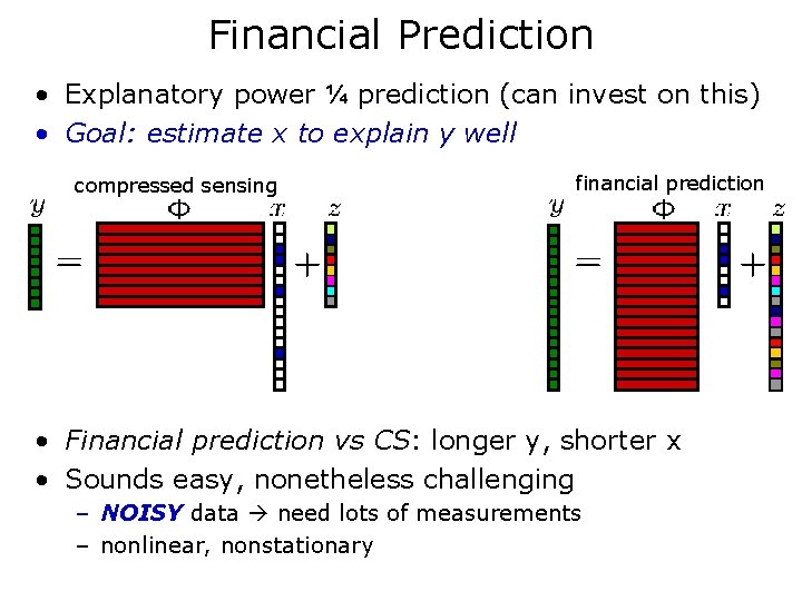
Financial Prediction • Explanatory power ¼ prediction (can invest on this) • Goal: estimate x to explain y well compressed sensing financial prediction • Financial prediction vs CS: longer y, shorter x • Sounds easy, nonetheless challenging – NOISY data need lots of measurements – nonlinear, nonstationary

Application Areas for Linear Measurements • DSP (CS) • Finance • Medical imaging (tomography) • Information retrieval • Seismic imaging (oil industry)

Unified Theory of Linear Measurement • Common goals – minimal resources – robustness – computationally tractable • Inverse problems • Striving toward theory and efficient processing in linear measurement systems

THE END