Lecture 13 Compressive sensing 1 Compressed Sensing A

Lecture 13 Compressive sensing 1

Compressed Sensing • A. k. a. compressive sensing or compressive sampling [Candes-Romberg-Tao’ 04; Donoho’ 04] • Signal acquisition/processing framework: – Want to acquire a signal x=[x 1…xn] – Acquisition proceeds by computing Ax of dimension m<<n (see next slide why) – From Ax we want to recover an approximation x* of x • Note: x* does not have to be k-sparse • Method: solve the following program: minimize ||x*||1 subject to Ax*=Ax

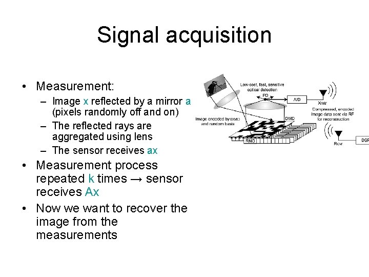
Signal acquisition • Measurement: – Image x reflected by a mirror a (pixels randomly off and on) – The reflected rays are aggregated using lens – The sensor receives ax • Measurement process repeated k times → sensor receives Ax • Now we want to recover the image from the measurements

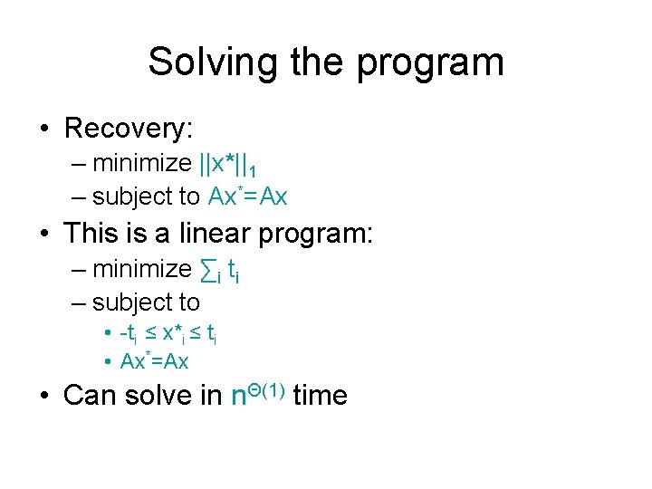
Solving the program • Recovery: – minimize ||x*||1 – subject to Ax*=Ax • This is a linear program: – minimize ∑i ti – subject to • -ti ≤ x*i ≤ ti • Ax*=Ax • Can solve in nΘ(1) time

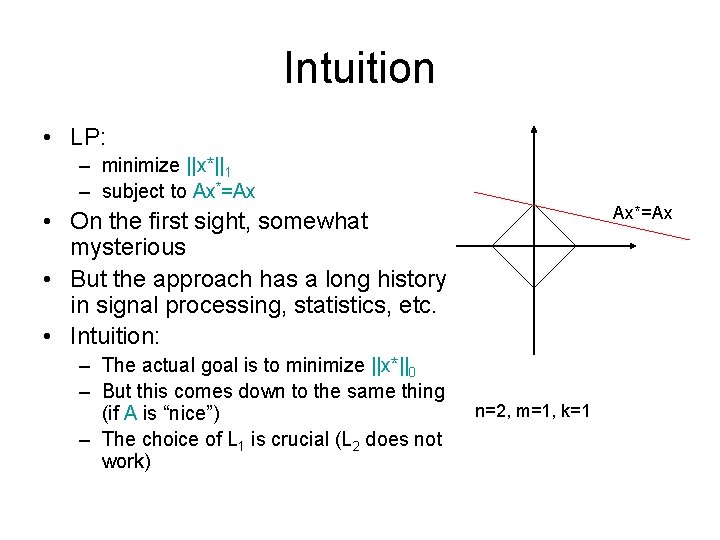
Intuition • LP: – minimize ||x*||1 – subject to Ax*=Ax • On the first sight, somewhat mysterious • But the approach has a long history in signal processing, statistics, etc. • Intuition: – The actual goal is to minimize ||x*||0 – But this comes down to the same thing (if A is “nice”) – The choice of L 1 is crucial (L 2 does not work) n=2, m=1, k=1

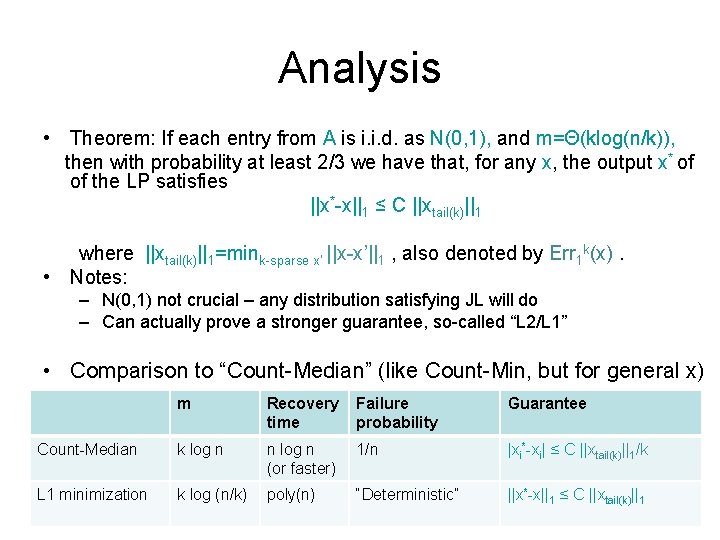
Analysis • Theorem: If each entry from A is i. i. d. as N(0, 1), and m=Θ(klog(n/k)), then with probability at least 2/3 we have that, for any x, the output x* of of the LP satisfies ||x*-x||1 ≤ C ||xtail(k)||1 where ||xtail(k)||1=mink-sparse x’ ||x-x’||1 , also denoted by Err 1 k(x). • Notes: – N(0, 1) not crucial – any distribution satisfying JL will do – Can actually prove a stronger guarantee, so-called “L 2/L 1” • Comparison to “Count-Median” (like Count-Min, but for general x) m Recovery time Failure probability Guarantee Count-Median k log n n log n (or faster) 1/n |xi*-xi| ≤ C ||xtail(k)||1/k L 1 minimization k log (n/k) poly(n) “Deterministic” ||x*-x||1 ≤ C ||xtail(k)||1

Empirical comparison • L 1 minimization more measurement-efficient • Sketching can be more time-efficient (sublinear in in)

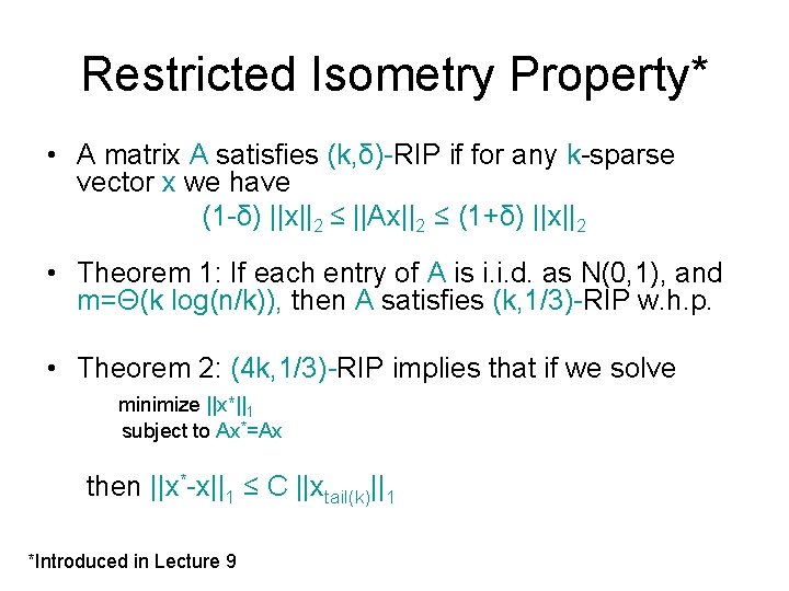
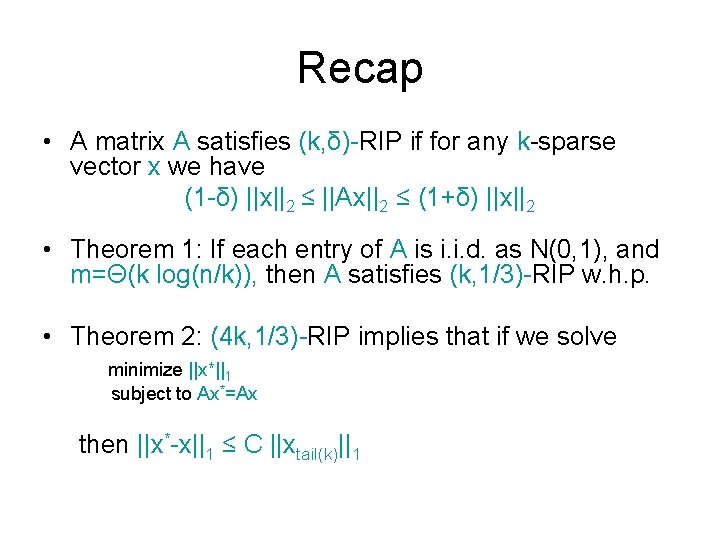
Restricted Isometry Property* • A matrix A satisfies (k, δ)-RIP if for any k-sparse vector x we have (1 -δ) ||x||2 ≤ ||Ax||2 ≤ (1+δ) ||x||2 • Theorem 1: If each entry of A is i. i. d. as N(0, 1), and m=Θ(k log(n/k)), then A satisfies (k, 1/3)-RIP w. h. p. • Theorem 2: (4 k, 1/3)-RIP implies that if we solve minimize ||x*||1 subject to Ax*=Ax then ||x*-x||1 ≤ C ||xtail(k)||1 *Introduced in Lecture 9

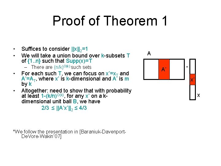
Proof of Theorem 1 • • Suffices to consider ||x||2=1 We will take a union bound over k-subsets T of {1. . n} such that Supp(x)=T – There are (n/k)O(k) such sets • • For each such T, we can focus on x’=x. T and A’=AT, where x’ is k-dimensional and A’ is m by k Altogether: need to show that with probability at least 1 -(k/n)O(k), for any x’ on a kdimensional unit ball B, we have 2/3 ≤ ||A’x’||2 ≤ 4/3 *We follow the presentation in [Baraniuk-Davenport. De. Vore-Wakin’ 07] A A’ * x’ x

Unit ball preservation • An ε-net N of B is a subset of B such that for any x’ B there is x” N s. t. ||x’-x”||2 < ε • Lect. 5: there exists an ε-net N for B of size (1/ε)Θ(k) – We set ε=1/7 • By JL we know that for all x’ N we have 7/8 ≤ ||A’x’||2 ≤ 8/7 with probability 1 -e-Θ(m) • To take care of all x’ B, we set x’=b 0 x 0+b 1 x 1+…, s. t. – All xj N – bj <1/7 j • We get – ||A’x’||2 ≤∑j ||Axj||/7 j ≤ 8/7 ∑j ||xj||/7 j =8/7*7/6=4/3 – Other direction analogous • Altogether, this gives us (1/3, k)-RIP with high probability Δ x’ x 0 …and recurse on Δ

Proof of Theorem 2 • See notes

Recap • A matrix A satisfies (k, δ)-RIP if for any k-sparse vector x we have (1 -δ) ||x||2 ≤ ||Ax||2 ≤ (1+δ) ||x||2 • Theorem 1: If each entry of A is i. i. d. as N(0, 1), and m=Θ(k log(n/k)), then A satisfies (k, 1/3)-RIP w. h. p. • Theorem 2: (4 k, 1/3)-RIP implies that if we solve minimize ||x*||1 subject to Ax*=Ax then ||x*-x||1 ≤ C ||xtail(k)||1