Dimensionality Reduction Principal Component Analysis slides adapted from

Dimensionality Reduction & Principal Component Analysis slides adapted from Princeton Picasso group

Clustering $$$ age Does this still work with high-dimensional data?

Recall: Curse of Dimensionality • Coined by Bellman in 1961 • Arises when analyzing and organizing data in high-dimensional spaces – Does not occur in low-dimensional settings • What is high-D? – high dimensional: hundreds, thousands of dimensions – low dimensional: usually <10

Principal Component Analysis (PCA) • Unsupervised learning method • Learns underlying factors that govern observed data • Often used for high-dimensional data – Example: Images (resolution 640 x 480) • ~300, 000 -D data • However, we can describe the content of images with much more compact feature representation • We want to identify and use the (low-d) latent factors rather than the (high-d) observed data

PCA Sketch Y • Provides low-D representation of data PCA 1 X – Finds linear correlations (xi, yi) (pi)

Basic Concept • If two dimensions (or attributes) are highly correlated – They are likely to represent highly related phenomena – If they tell us about the same underlying variance in the data, combining them to form a single measure may be reasonable • We want a smaller set of variables that explain most of the variance in the original data – In more compact and insightful form

Basic Concept (cont’d) • What if the dependences and correlations are not so strong or direct? • And suppose you have 3 variables, or 4, or 5, or 10000? • Look for the phenomena underlying the observed covariance/co-dependence in a set of variables – Once again, phenomena that are uncorrelated or independent, and especially those along which the data show high variance • These phenomena are called factors or principal components

Principal Component Analysis • Most common form of factor analysis • New variables/dimensions – Are linear combinations of the original ones – Are uncorrelated with one another • Orthogonal in original dimension space – Capture as much of the original variance in the data as possible – Are called Principal Components

• First principal component is the direction of greatest variability (covariance) in the data • Second is the next orthogonal (uncorrelated) direction of greatest variability – So first remove all the variability along the first component, and then find the next direction of greatest variability • And so on … Original Variable B Principal Components PC 2 PC 1 Original Variable A

Computing the Components • Projection of vector x onto an axis (dimension) u is ux • Direction of greatest variability is that in which the average square of the projection is greatest – I. e. u such that E((ux)2) over all x is maximized • Note: We subtract the mean along each dimension, and center the original axis system at the centroid of all data points, for simplicity – This direction of u is the direction of the first Principal Component

Computing the Components • E((ux)2) = E ((ux)T) = E (u. Txx Tu) The matrix C = xx. T contains the correlations of the original axes • Maximize u. Txx. Tu such that u. Tu = 1 • Construct Lagrangian u. Txx. Tu – λu. Tu • Vector of partial derivatives set to zero – xx. Tu – λu = (xx. T – λI) u = 0 • As u ≠ 0 then u must be an eigenvector of xx. T with eigenvalue λ • Can we find these eigenvectors quickly?

1 -dimensional k-dimensional

Singular Value Decomposition (SVD) • The first root is called the principal eigenvalue which has an associated eigenvector u • Subsequent roots are ordered such that λ 1> λ 2 >… > λM

SVD (cont’d) • The eigenvalue decomposition of xx. T = UΣUT – where U = [u 1, u 2, …, u. M] – and Σ = diag[λ 1, λ 2, …, λ M] • Similarly, x. Tx = VΣVT • The SVD is closely related to the above: x=U Σ 1/2 VT • The left eigenvectors U, right eigenvectors V • singular values = square root of eigenvalues

Computing the Components • So, the new axes are the eigenvectors of the matrix of correlations of the original variables – Captures the similarities of the original variables based on how data samples project to them n Geometrically: centering followed by rotation ¨ Linear transformation

PCs, Variance and Least-Squares • The first PC retains the greatest amount of variation in the sample • The kth PC retains the kth greatest fraction of the variation in the sample • The kth largest eigenvalue of the correlation matrix C is the variance in the sample along the kth PC • The least-squares view: PCs are a series of linear least squares fits to a sample, each orthogonal to all previous ones

How Many Principal Components? • For n original dimensions, correlation matrix is nxn, and has up to n eigenvectors. – So n Principal Components – Can this be less than n? greater? • Where does dimensionality reduction come from?

Dimensionality Reduction • Can ignore the components of lesser significance • You do lose some information, but if the eigenvalues are small, you don’t lose much – – n dimensions in original data calculate n eigenvectors and eigenvalues choose only the first p eigenvectors, based on their eigenvalues final data set has only p dimensions

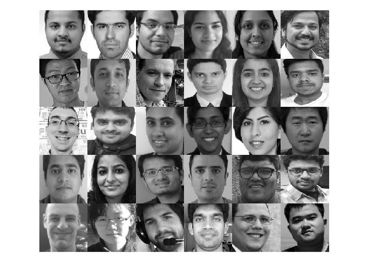
PCA with Image Data: Eigenfaces • Input: Digital Images of Faces • Goal: Usual machine learning problems – Is this a picture of Joe? (Classification) – Are these pictures of the same person? (Clustering) • Eigenfaces: Algorithm used to model image data (of human faces) • Why PCA? – To model the (low-d) latent parameters that correspond to the (highd) images – Eigenfaces are the ‘standardized face ingredients’ derived from the statistical analysis of many pictures of human faces – A human face may be considered to be a combination of these standard faces

Eigenfaces Low Dimensional Representation PCA = a 1 × + a 2 × + a 3 × + a 4 × + + an×

Centering the Data • Computing the mean of the data set • This is the “average” image – The average intensity at each pixel location • For a large enough group of people, this type of “ghost” is a common average

PCA Input = Original - Average

Linear Combinations of Images • For this data set, these are the (first three) principal components: • Recall that a principal component is a vector in feature space • If the feature vectors are images, the principal components can be viewed as images

Eigenfaces: Dimensionality Reduction • Eigenfaces provide a means of applying data compression (dimensionality reduction) to faces for identification purposes – Input: Image (high-dimensional, # of pixels) – Output: (low-d) vector of PCA coordinates • Eigenfaces can be summed together to create an approximate rendering of a human face

Eigenfaces: Dimensionality Reduction • We can represent an image as the avg. image + “how much of each principal vector it uses” 6. 30 = -1. 61 -4. 23 + Avg Image = 1. 79 1. 13 0. 63

Eigenfaces: Reconstruction What does this combination look like? 6. 30 -1. 61 -4. 23 = + Avg Image 1. 79 1. 13 0. 63 =

Eigenfaces for Recognition • ORL database of faces – Facial images of 16 persons each with 10 views are used • Variations in lighting and facial expression – Training set contains 16× 7 images. – Test set contains 16× 3 images • First three eigenfaces :

Classification: PCA + 1 -NN • Save average coefficients for each person • Classify new face as the person with the closest average • Recognition accuracy increases with number of eigenfaces – Plateau around 15 – Later eigenfaces do not help much with recognition Recognition rates d=1 78% d = 15 89% d = 50 89%

Eigenfaces Summary • Developed in 1987 for face recognition – Pre-processing required • Same resolution for all data, align eyes, etc. – More sophisticated methods exist now • (Visual) example of PCA for dimensionality reduction

Notes on PCA • PCA is not the most sophisticated dimensionality reduction technique • Have we already learned others? – Neural nets, support vector machines etc. • Dimensionality reduction / feature selection is implicit for many PRML methods

PCA Alternatives Are the maximal variance dimensions always the most relevant dimensions? • Relevant Component Analysis (RCA) • Fisher Discriminant analysis (FDA)

PCA vs ICA PCA (orthogonal coordinate) ICA (non-orthogonal coordinate)

Summary • PCA – Linear Dimensionality Reduction – Used for high-dimensional data – For PRML, can be considered as: • Learning latent variables • Pre-processing step to avoid “curse of dimensionality” – Treat coefficients as input data • There are nonlinear variants of this idea – We can formulate PCA using only dot products between input points… (any ideas? )