Principal Component Analysis Principal components analysis is similar

Principal Component Analysis

Principal components analysis is similar to factor analysis in that it is a technique for examining the interrelationships among a set of variables. Both of these techniques differ from regression analysis in that we do not have a dependent variable to be explained by a set of independent variables. However, principal components analysis and factor analysis also differ from each other. In principal components analysis the major objective is to select a number of components that explain as much of the total variance as possible, that is, in PCA one is simply trying to statistically derive a relatively small number of variables. The values of the principal components for a given individual are relatively simple to compute and interpret. On the other hand, the factors obtained in factor analysis are selected mainly to explain the interrelationships among the original variables. Ideally, in exploratory factor analysis the number of factors expected is known in advance. The major emphasis is placed on obtaining easily understandable factors that convey the essential information contained in the original set of variables. Ordinary principal axis factor analysis should NOT be done if the number of Variables > the number of Participants.

When is principal components analysis used? Principal components analysis is performed in order to simplify the description of a set of interrelated variables. Each principal component is a linear combination of the original variables. One measure of the amount of information conveyed by each principal component is its variance. For this reason the principal components are arranged in order of decreasing variance. Thus the most informative principal component is the first, and the least informative is the last (a variable with zero variance does not distinguish between the members of the population).

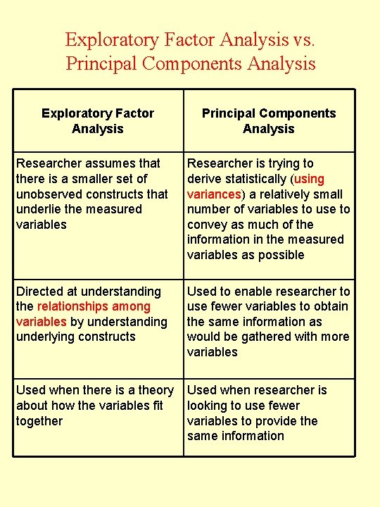
Exploratory Factor Analysis vs. Principal Components Analysis Exploratory Factor Analysis Principal Components Analysis Researcher assumes that there is a smaller set of unobserved constructs that underlie the measured variables Researcher is trying to derive statistically (using variances) a relatively small number of variables to use to convey as much of the information in the measured variables as possible Directed at understanding the relationships among variables by understanding underlying constructs Used to enable researcher to use fewer variables to obtain the same information as would be gathered with more variables Used when there is a theory about how the variables fit together Used when researcher is looking to use fewer variables to provide the same information

Assumptions • Normality – Important only to the extent that skewness/outliers affect observed correlations – OR if significance tests are performed (rare) • Independent sampling required • Variables should be linearly related to one another (in pairs) • Many of the variables should be correlated at a moderate level (test with Bartlett’s test of sphericity)

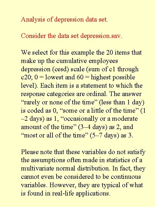
Analysis of depression data set. Consider the data set depression. sav. We select for this example the 20 items that make up the cumulative employees depression (cesd) scale (sum of c 1 through c 20; 0 = lowest and 60 = highest possible level). Each item is a statement to which the response categories are ordinal. The answer “rarely or none of the time” (less than 1 day) is coded as 0, “some or a little of the time” (1 – 2 days) as 1, “occasionally or a moderate amount of the time” (3– 4 days) as 2, and “most or all of the time” (5– 7 days) as 3. Please note that these variables do not satisfy the assumptions often made in statistics of a multivariate normal distribution. In fact, they cannot even be considered to be continuous variables. However, they are typical of what is found in real-life applications.

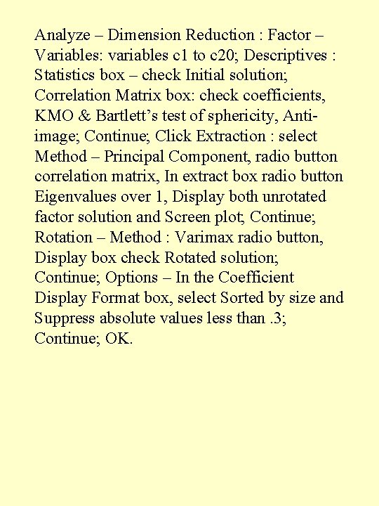
Analyze – Dimension Reduction : Factor – Variables: variables c 1 to c 20; Descriptives : Statistics box – check Initial solution; Correlation Matrix box: check coefficients, KMO & Bartlett’s test of sphericity, Antiimage; Continue; Click Extraction : select Method – Principal Component, radio button correlation matrix, In extract box radio button Eigenvalues over 1, Display both unrotated factor solution and Screen plot; Continue; Rotation – Method : Varimax radio button, Display box check Rotated solution; Continue; Options – In the Coefficient Display Format box, select Sorted by size and Suppress absolute values less than. 3; Continue; OK.

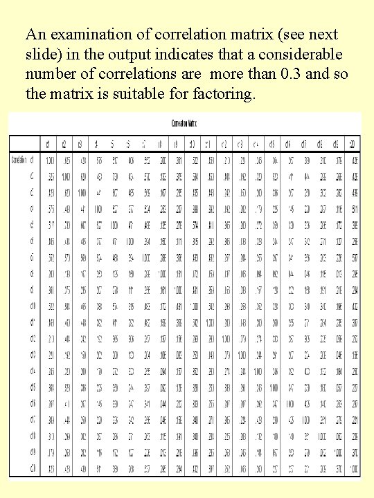
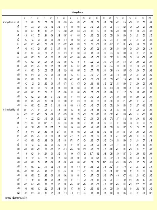
An examination of correlation matrix (see next slide) in the output indicates that a considerable number of correlations are more than 0. 3 and so the matrix is suitable for factoring.

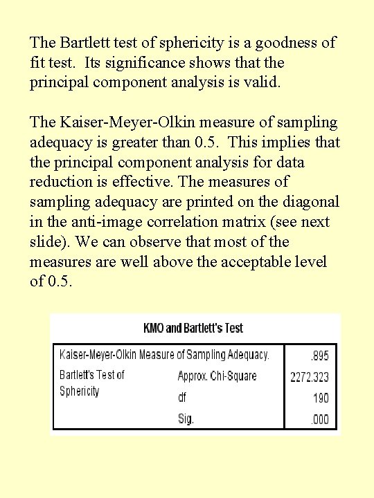
The Bartlett test of sphericity is a goodness of fit test. Its significance shows that the principal component analysis is valid. The Kaiser-Meyer-Olkin measure of sampling adequacy is greater than 0. 5. This implies that the principal component analysis for data reduction is effective. The measures of sampling adequacy are printed on the diagonal in the anti-image correlation matrix (see next slide). We can observe that most of the measures are well above the acceptable level of 0. 5.

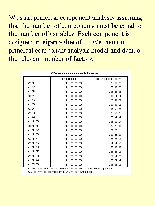
We start principal component analysis assuming that the number of components must be equal to the number of variables. Each component is assigned an eigen value of 1. We then run principal component analysis model and decide the relevant number of factors.

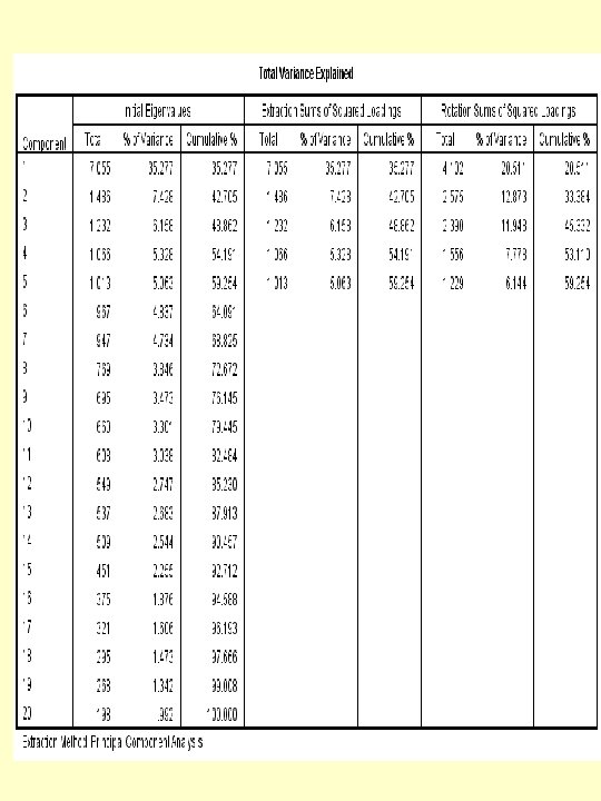
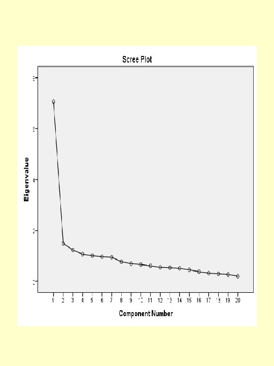
The table of Total Variance Explained displays the total variance explained in three stages. At the initial stage, it shows that the components and their associated eigenvalues, the percentage of variance explained and the cumulative percentages. In reference to eigenvalues, we would expect that five components to be extracted because they have eigenvalues greater than 1. If five factors were extracted, then 59% of the variance would be explained. The screen plot graphically displays the eigenvalues for each component.

It should be explained that the eigenvalues are estimated variances of the principal components and are therefore subject to large sample variations. Thus, arbitrary cutoff points should not be taken too seriously. Once the number of principal components is selected, the investigator should examine the coefficients defining each of them in order to assign an interpretation to the components. A high coefficient of a principal component on a given variable is an indication of high correlation between that variable and the principal component. Principal components are interpreted in the context of the variables with high coefficients. Component Transformation Matrix - This is the matrix by which you multiply the unrotated component matrix to get the rotated component matrix.

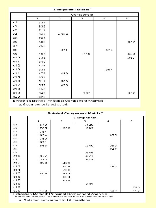
The component matrix is the matrix of loadings or correlations between the variables and components. Pure variables have loadings of 0. 3 or greater on only one component. Complex variables may have high loadings on more than one component, and they make interpretation of the output difficult. Rotation may therefore be necessary. Varimax rotation, where the component axes are kept at right angles to each other, is the most frequently chosen. Ordinarily, rotation reduces the number of complex variables and improves interpretation. component 1 comprises of 7 items. Component 2 comprises of 6 items, component 3 comprises of 4 items, component 4 consists of 2 items and component 5 consists of 1 item. Some items have dual (or sometimes triple/multiple) loadings greater than 0. 3 on more than one component. These items must be interpreted with caution, because simple structure in not apparent.

The depression data example illustrates a situation in which the results are not clear-cut. The conclusion may be reached from observing screen plot Figure, where we see that it is difficult to decide how many components to use. It is not possible to explain a very high proportion of the total variance with a small number of principal components. Also, the interpretation of the components is not straightforward. This is frequently the case in real-life situations.