Development of Verification and Validation Procedures for Computer

Development of Verification and Validation Procedures for Computer Simulation use in Roadside Safety Applications NCHRP 22 -24 VERIFICATION AND VALIDTION METRICS Worcester Polytechnic Institute Battelle Memorial Laboratory Politecnico di Milano

Meeting Agenda 9: 00 -9: 30 -10: 30 -11: 30 -Noon-1: 00 - 2: 30 -4: 00 Introductions/Instructions (Niessner, Focke) Definitions and V&V Procedures (Ray) ROBUST Project Summary (Anghileri) Survey Results Lunch V&V Metrics (Ray) Future Work for Task 8 (Ray)

BACKGROUND • Validation and verification metrics: – Quantify the level of agreement between two solutions. – Calculate the error (i. e. , difference) between two solutions. • Specification and use of validation/verification metrics is important because different metrics give different scores for the same time-history pairs. • Need an automated, consistent, repeatable, non -subjective procedure.

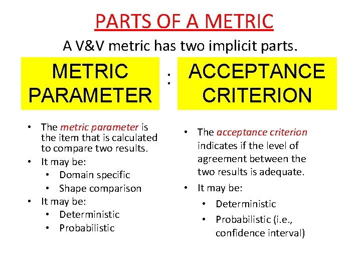
PARTS OF A METRIC A V&V metric has two implicit parts. METRIC : ACCEPTANCE PARAMETER CRITERION • The metric parameter is the item that is calculated to compare two results. • It may be: • Domain specific • Shape comparison • It may be: • Deterministic • Probabilistic • The acceptance criterion indicates if the level of agreement between the two results is adequate. • It may be: • Deterministic • Probabilistic (i. e. , confidence interval)

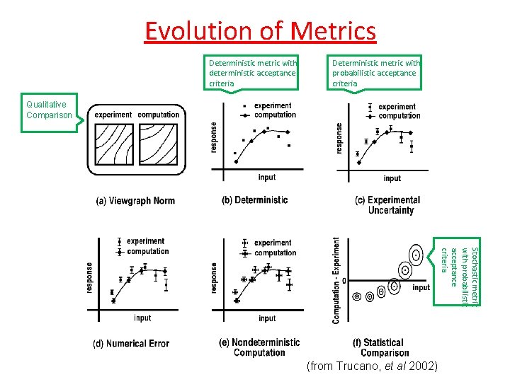
Evolution of Metrics Deterministic metric with deterministic acceptance criteria Deterministic metric with probabilistic acceptance criteria Qualitative Comparison Stochastic metric with probabilistic acceptance criteria (from Trucano, et al 2002)

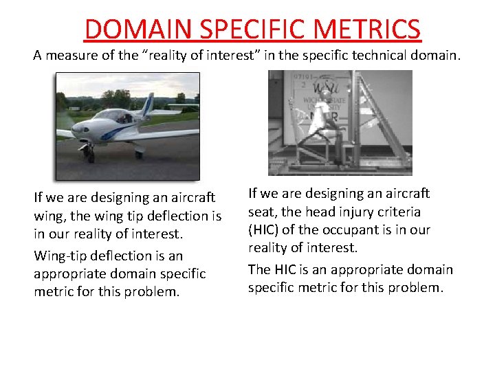
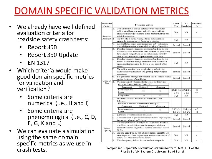
DOMAIN SPECIFIC METRICS A measure of the “reality of interest” in the specific technical domain. If we are designing an aircraft wing, the wing tip deflection is in our reality of interest. Wing-tip deflection is an appropriate domain specific metric for this problem. If we are designing an aircraft seat, the head injury criteria (HIC) of the occupant is in our reality of interest. The HIC is an appropriate domain specific metric for this problem.

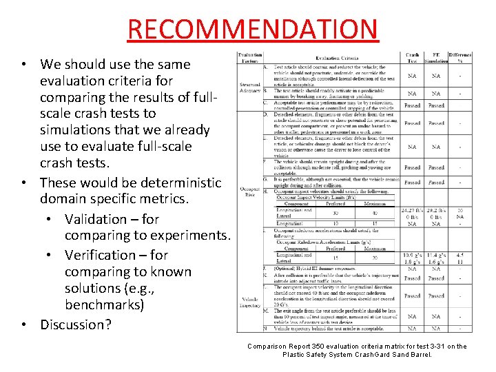
DOMAIN SPECIFIC VALIDATION METRICS • We already have well defined evaluation criteria for roadside safety crash tests: • Report 350 Update • EN 1317 • Which criteria would make good domain specific metrics for validation and verification? • Some criteria are numerical (i. e. , H and I) • Some criteria are phenomological (i. e. , C, D, F, G, K and L) • We can evaluate a simulation using the same domain specific metrics as we use in crash tests. Comparison Report 350 evaluation criteria matrix for test 3 -31 on the Plastic Safety System Crash. Gard Sand Barrel.

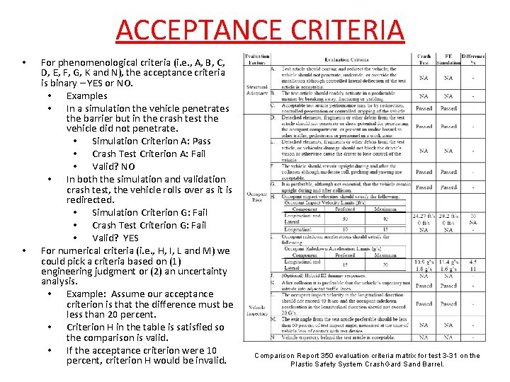
RECOMMENDATION • We should use the same evaluation criteria for comparing the results of fullscale crash tests to simulations that we already use to evaluate full-scale crash tests. • These would be deterministic domain specific metrics. • Validation – for comparing to experiments. • Verification – for comparing to known solutions (e. g. , benchmarks) • Discussion? Comparison Report 350 evaluation criteria matrix for test 3 -31 on the Plastic Safety System Crash. Gard Sand Barrel.

ACCEPTANCE CRITERIA • • For phenomenological criteria (i. e. , A, B, C, D, E, F, G, K and N), the acceptance criteria is binary – YES or NO. • Examples • In a simulation the vehicle penetrates the barrier but in the crash test the vehicle did not penetrate. • Simulation Criterion A: Pass • Crash Test Criterion A: Fail • Valid? NO • In both the simulation and validation crash test, the vehicle rolls over as it is redirected. • Simulation Criterion G: Fail • Crash Test Criterion G: Fail • Valid? YES For numerical criteria (i. e. , H, I, L and M) we could pick a criteria based on (1) engineering judgment or (2) an uncertainty analysis. • Example: Assume our acceptance criterion is that the difference must be less than 20 percent. • Criterion H in the table is satisfied so the comparison is valid. • If the acceptance criterion were 10 percent, criterion H would be invalid. Comparison Report 350 evaluation criteria matrix for test 3 -31 on the Plastic Safety System Crash. Gard Sand Barrel.

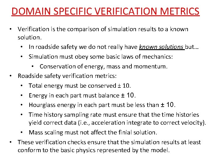
DOMAIN SPECIFIC VERIFICATION METRICS • Verification is the comparison of simulation results to a known solution. • In roadside safety we do not really have known solutions but… • Simulation must obey some basic laws of mechanics: • Conservation of energy, mass and momentum. • Roadside safety verification metrics: • Total energy must be conserved ± 10. • Energy in each part must balance ± 10. • Hourglass energy in each part must be less than ± 10. • Time history sampling rate must ensure that the time histories yield correct data (i. e. , acceleration integrate to correct velocity). • Mass scaling must not affect the finial solution. • These verification checks ensure that the simulation results at least conform to the basic physics represented by the model.

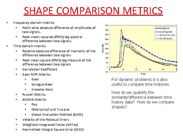
SHAPE COMPARISON METRICS • • Frequency domain metrics • Point-wise absolute difference of amplitudes of two signals. • Root-mean-squared (RMS) log spectral difference between two signals. Time domain metrics • Relative absolute difference of moments of the difference between two signals • Root mean square (RMS) log measure of the difference between two signals • Correlation Coefficient • Geer MPC Metrics • Geer • Sprague-Geer • Knowles-Gear • Russell Metrics • ANOVA Metrics • Ray • Oberkampf and Trucano • Global Evaluation Method (GEM) • Velocity of the Residual Errors • Weighted Integrated Factor (WIFac) • Normalized Integral Square Error (NISE) For dynamic problems it is also useful to compare time histories. How do we quantify the similarity/difference between time history data? How do we compare shapes?

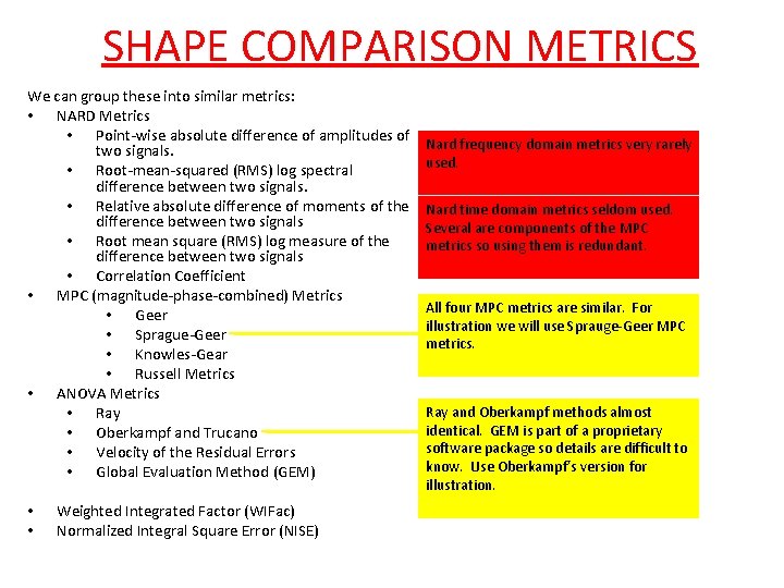
SHAPE COMPARISON METRICS We can group these into similar metrics: • NARD Metrics • Point-wise absolute difference of amplitudes of two signals. • Root-mean-squared (RMS) log spectral difference between two signals. • Relative absolute difference of moments of the difference between two signals • Root mean square (RMS) log measure of the difference between two signals • Correlation Coefficient • MPC (magnitude-phase-combined) Metrics • Geer • Sprague-Geer • Knowles-Gear • Russell Metrics • ANOVA Metrics • Ray • Oberkampf and Trucano • Velocity of the Residual Errors • Global Evaluation Method (GEM) • • Weighted Integrated Factor (WIFac) Normalized Integral Square Error (NISE) Nard frequency domain metrics very rarely used. Nard time domain metrics seldom used. Several are components of the MPC metrics so using them is redundant. All four MPC metrics are similar. For illustration we will use Sprauge-Geer MPC metrics. Ray and Oberkampf methods almost identical. GEM is part of a proprietary software package so details are difficult to know. Use Oberkampf’s version for illustration.

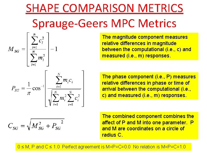
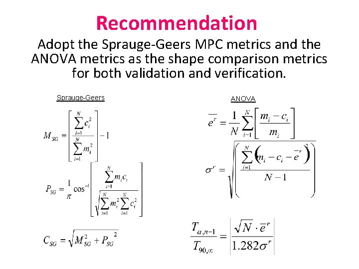
SHAPE COMPARISON METRICS Sprauge-Geers MPC Metrics The magnitude component measures relative differences in magnitude between the computational (i. e. , c) and measured (i. e. , m) responses. The phase component (i. e. , P) measures relative differences in phase or time of arrival between the computational (i. e. , c) and measured (i. e. , m) responses. The combined component combines the affect of P and M into one parameter. P and M are coordinates on a circle of radius C. 0 ≤ M, P and C ≤ 1. 0 Perfect agreement is M=P=C=0. 0 No relation is M=P=C=1. 0

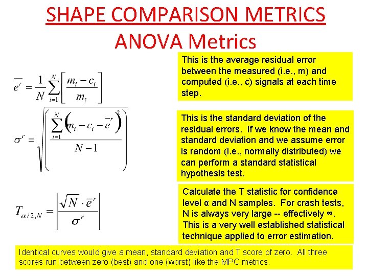
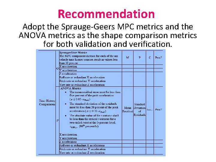
SHAPE COMPARISON METRICS ANOVA Metrics This is the average residual error between the measured (i. e. , m) and computed (i. e. , c) signals at each time step. This is the standard deviation of the residual errors. If we know the mean and standard deviation and we assume error is random (i. e. , normally distributed) we can perform a standard statistical hypothesis test. Calculate the T statistic for confidence level α and N samples. For crash tests, N is always very large -- effectively ∞. This is a very well established statistical technique applied to error estimation. Identical curves would give a mean, standard deviation and T score of zero. All three scores run between zero (best) and one (worst) like the MPC metrics.

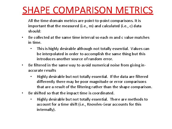
SHAPE COMPARISON METRICS • • • All the time-domain metrics are point-to-point comparisons. It is important that the measured (i. e. , m) and calculated (i. e. , c) data should: Be collected at the same time interval so each m and c value matches in time. • This is highly desirable although not totally essential. Values can be interpolated in order to accomplish the same thing but this introduces another source of random error. Be filtered in the same way to avoid numerical noise from giving inaccurate results • Highly desirable but not totally essential. If the data are filtered differently there may be poor magnitude or error comparisons that are a result of the filtering rather than the shape comparison. Be shifted so that the impact time is coordinated. • Highly desirable but not totally essential. There are methods to account for a time shift (i. e. , Knowles-Gear accounts for this internally).

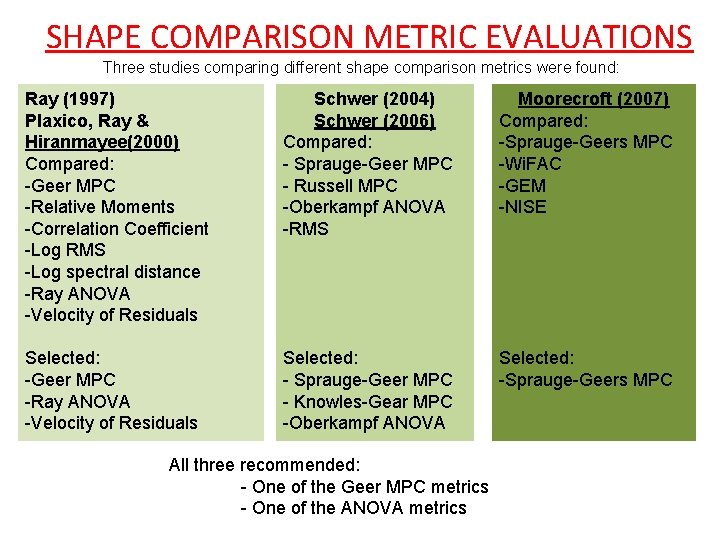
SHAPE COMPARISON METRIC EVALUATIONS Three studies comparing different shape comparison metrics were found: Ray (1997) Plaxico, Ray & Hiranmayee(2000) Compared: -Geer MPC -Relative Moments -Correlation Coefficient -Log RMS -Log spectral distance -Ray ANOVA -Velocity of Residuals Schwer (2004) Schwer (2006) Compared: - Sprauge-Geer MPC - Russell MPC -Oberkampf ANOVA -RMS Moorecroft (2007) Compared: -Sprauge-Geers MPC -Wi. FAC -GEM -NISE Selected: -Geer MPC -Ray ANOVA -Velocity of Residuals Selected: - Sprauge-Geer MPC - Knowles-Gear MPC -Oberkampf ANOVA Selected: -Sprauge-Geers MPC All three recommended: - One of the Geer MPC metrics - One of the ANOVA metrics

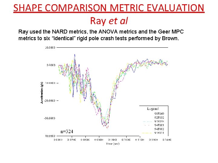
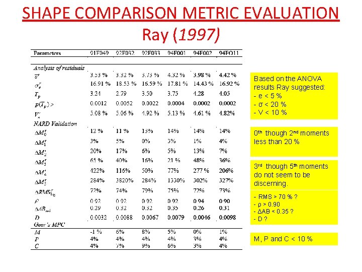
SHAPE COMPARISON METRIC EVALUATION Ray et al Ray used the NARD metrics, the ANOVA metrics and the Geer MPC metrics to six “identical” rigid pole crash tests performed by Brown.

SHAPE COMPARISON METRIC EVALUATION Ray (1997) Based on the ANOVA results Ray suggested: -e<5% - σ < 20 % - V < 10 % 0 th though 2 nd moments less than 20 % 3 rd though 5 th moments do not seem to be discerning. - RMS > 70 % ? - ρ > 0. 90 - ΔAB < 0. 35 ? -D? M, P and C < 10 %

SHAPE COMPARISON METRIC EVALUATION Schwer • Schwer examined four metrics: – Oberkampf’s version of the ANOVA metrics – Sprauge-Geers MPC metrics – Russell metrics – Root-mean square (RMS) metric • Results should be consistent with Subject Matter Expert (SME) opinions. • Increased use of metrics, but selection rationale is rarely specified.

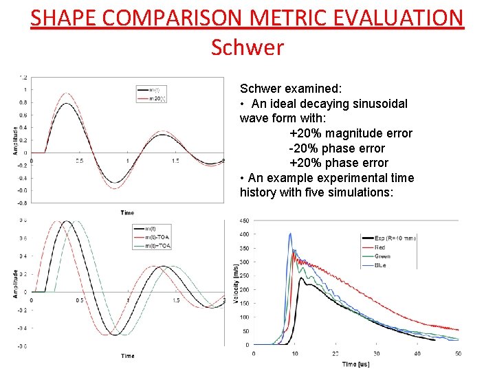
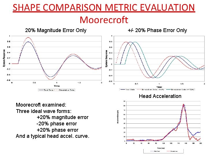
SHAPE COMPARISON METRIC EVALUATION Schwer examined: • An ideal decaying sinusoidal wave form with: +20% magnitude error -20% phase error +20% phase error • An example experimental time history with five simulations:

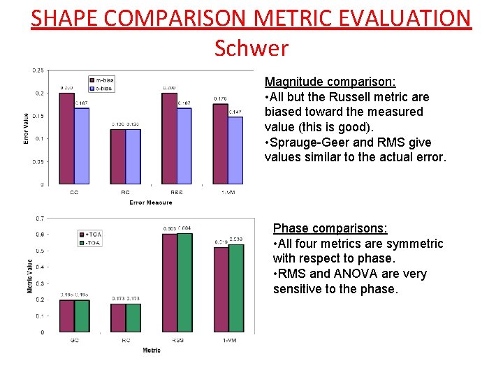
SHAPE COMPARISON METRIC EVALUATION Schwer Magnitude comparison: • All but the Russell metric are biased toward the measured value (this is good). • Sprauge-Geer and RMS give values similar to the actual error. Phase comparisons: • All four metrics are symmetric with respect to phase. • RMS and ANOVA are very sensitive to the phase.

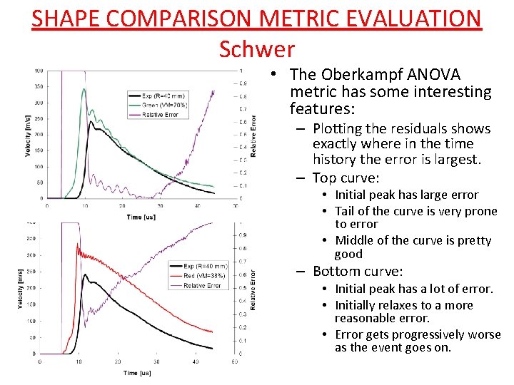
SHAPE COMPARISON METRIC EVALUATION Schwer • The Oberkampf ANOVA metric has some interesting features: – Plotting the residuals shows exactly where in the time history the error is largest. – Top curve: • Initial peak has large error • Tail of the curve is very prone to error • Middle of the curve is pretty good – Bottom curve: • Initial peak has a lot of error. • Initially relaxes to a more reasonable error. • Error gets progressively worse as the event goes on.

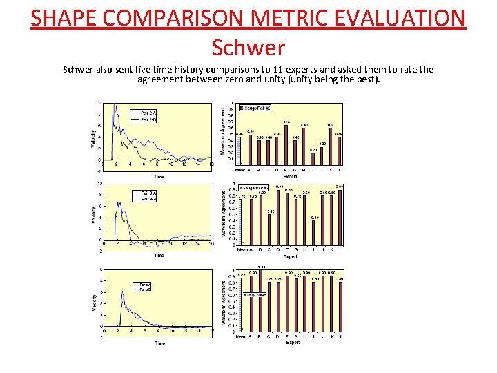
SHAPE COMPARISON METRIC EVALUATION Schwer also sent five time history comparisons to 11 experts and asked them to rate the agreement between zero and unity (unity being the best).

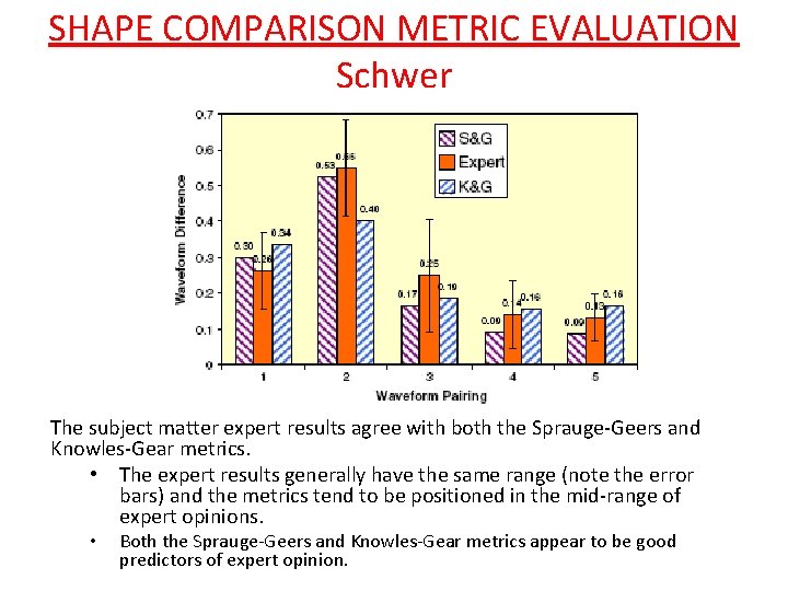
SHAPE COMPARISON METRIC EVALUATION Schwer The subject matter expert results agree with both the Sprauge-Geers and Knowles-Gear metrics. • The expert results generally have the same range (note the error bars) and the metrics tend to be positioned in the mid-range of expert opinions. • Both the Sprauge-Geers and Knowles-Gear metrics appear to be good predictors of expert opinion.

SHAPE COMPARISON METRIC EVALUATION Moorecroft Four Curve Shape Metrics Evaluated • Sprague and Geers (S&G) – General purpose curve shape metric – Implemented in a spreadsheet • Weighted Integrated Factor (WIFac) – Automotive curve shape metric – Implemented in a spreadsheet • Global Evaluation Method (GEM) – Automotive curve shape plus peak and timing – Requires Mod. Eval (stand alone program) • Normalized Integral Square Error (NISE) – Biomechanics curve shape plus magnitude and phase – Implemented in a spreadsheet

SHAPE COMPARISON METRIC EVALUATION Moorecroft 20% Magnitude Error Only +/- 20% Phase Error Only Head Acceleration Moorecroft examined: Three ideal wave forms: +20% magnitude error -20% phase error +20% phase error And a typical head accel. curve.

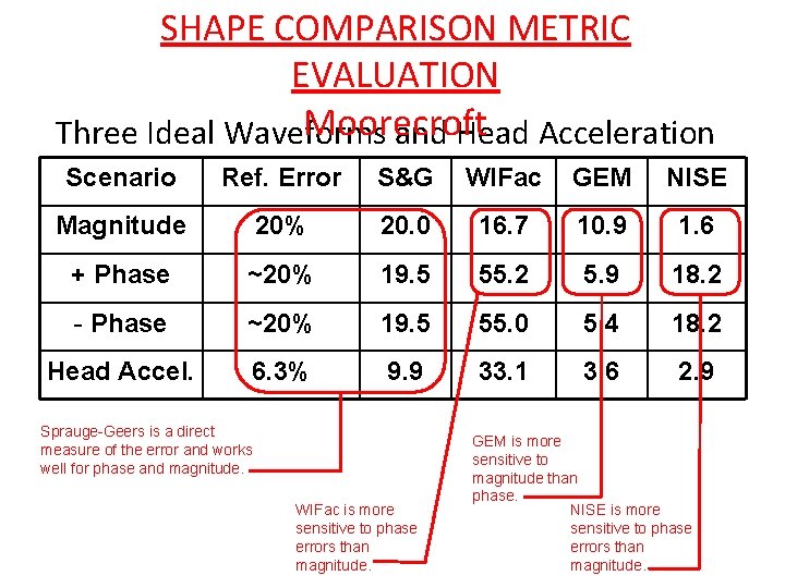
SHAPE COMPARISON METRIC EVALUATION Moorecroft Three Ideal Waveforms and Head Acceleration Scenario Ref. Error S&G WIFac GEM NISE Magnitude 20% 20. 0 16. 7 10. 9 1. 6 + Phase ~20% 19. 5 55. 2 5. 9 18. 2 - Phase ~20% 19. 5 55. 0 5. 4 18. 2 Head Accel. 6. 3% 9. 9 33. 1 3. 6 2. 9 Sprauge-Geers is a direct measure of the error and works well for phase and magnitude. WIFac is more sensitive to phase errors than magnitude. GEM is more sensitive to magnitude than phase. NISE is more sensitive to phase errors than magnitude.

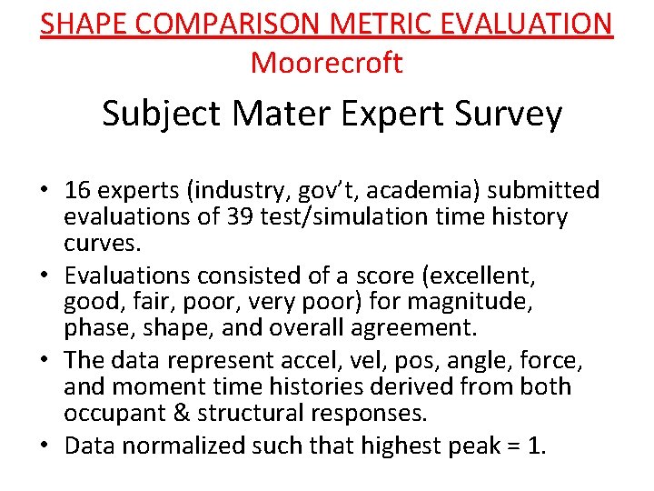
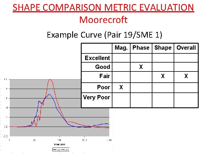
SHAPE COMPARISON METRIC EVALUATION Moorecroft Subject Mater Expert Survey • 16 experts (industry, gov’t, academia) submitted evaluations of 39 test/simulation time history curves. • Evaluations consisted of a score (excellent, good, fair, poor, very poor) for magnitude, phase, shape, and overall agreement. • The data represent accel, vel, pos, angle, force, and moment time histories derived from both occupant & structural responses. • Data normalized such that highest peak = 1.

SHAPE COMPARISON METRIC EVALUATION Moorecroft Example Curve (Pair 19/SME 1) Mag. Phase Shape Overall Excellent Good X Fair Poor Very Poor X X X

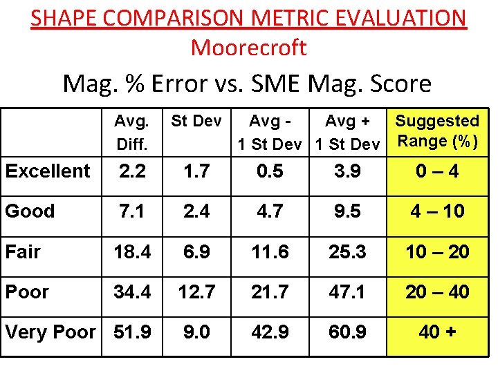
SHAPE COMPARISON METRIC EVALUATION Moorecroft Mag. % Error vs. SME Mag. Score Avg. Diff. St Dev Avg + Suggested 1 St Dev Range (%) Excellent 2. 2 1. 7 0. 5 3. 9 0– 4 Good 7. 1 2. 4 4. 7 9. 5 4 – 10 Fair 18. 4 6. 9 11. 6 25. 3 10 – 20 Poor 34. 4 12. 7 21. 7 47. 1 20 – 40 Very Poor 51. 9 9. 0 42. 9 60. 9 40 +

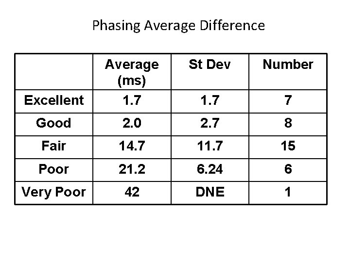
Phasing Average Difference St Dev Number Excellent Average (ms) 1. 7 7 Good 2. 0 2. 7 8 Fair 14. 7 11. 7 15 Poor 21. 2 6. 24 6 Very Poor 42 DNE 1

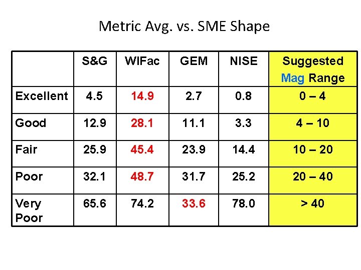
Metric Avg. vs. SME Shape S&G WIFac GEM NISE Excellent 4. 5 14. 9 2. 7 0. 8 Suggested Mag Range 0– 4 Good 12. 9 28. 1 11. 1 3. 3 4 – 10 Fair 25. 9 45. 4 23. 9 14. 4 10 – 20 Poor 32. 1 48. 7 31. 7 25. 2 20 – 40 Very Poor 65. 6 74. 2 33. 6 78. 0 > 40

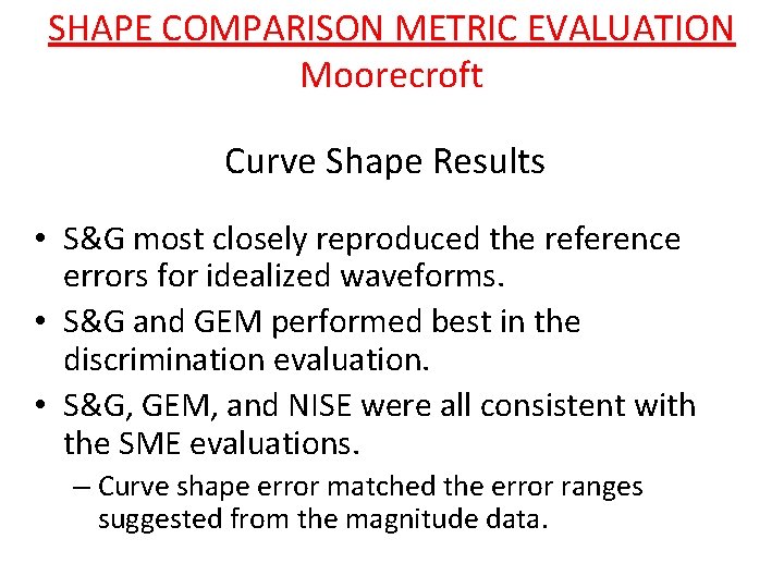
SHAPE COMPARISON METRIC EVALUATION Moorecroft Curve Shape Results • S&G most closely reproduced the reference errors for idealized waveforms. • S&G and GEM performed best in the discrimination evaluation. • S&G, GEM, and NISE were all consistent with the SME evaluations. – Curve shape error matched the error ranges suggested from the magnitude data.

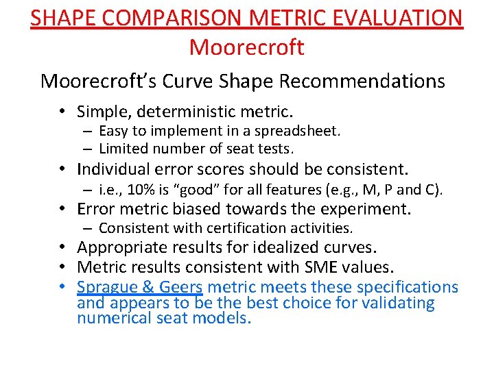
SHAPE COMPARISON METRIC EVALUATION Moorecroft’s Curve Shape Recommendations • Simple, deterministic metric. – Easy to implement in a spreadsheet. – Limited number of seat tests. • Individual error scores should be consistent. – i. e. , 10% is “good” for all features (e. g. , M, P and C). • Error metric biased towards the experiment. – Consistent with certification activities. • Appropriate results for idealized curves. • Metric results consistent with SME values. • Sprague & Geers metric meets these specifications and appears to be the best choice for validating numerical seat models.

Recommendation Adopt the Sprauge-Geers MPC metrics and the ANOVA metrics as the shape comparison metrics for both validation and verification. Sprauge-Geers ANOVA

Recommendation Adopt the Sprauge-Geers MPC metrics and the ANOVA metrics as the shape comparison metrics for both validation and verification.

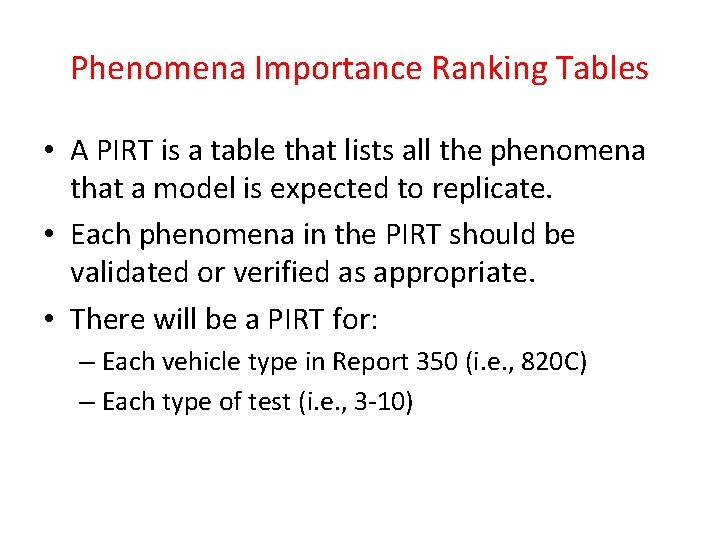
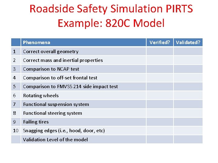
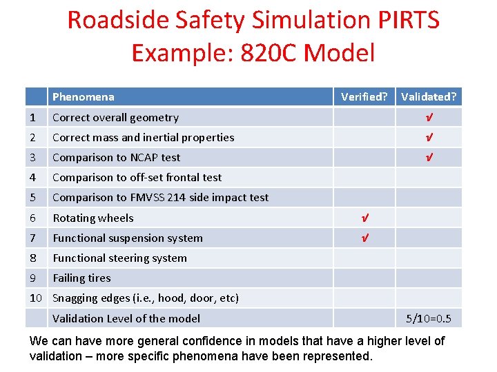
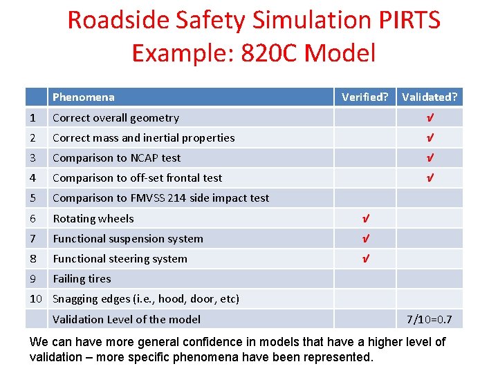
Phenomena Importance Ranking Tables • A PIRT is a table that lists all the phenomena that a model is expected to replicate. • Each phenomena in the PIRT should be validated or verified as appropriate. • There will be a PIRT for: – Each vehicle type in Report 350 (i. e. , 820 C) – Each type of test (i. e. , 3 -10)

Roadside Safety Simulation PIRTS Example: 820 C Model Phenomena 1 Correct overall geometry 2 Correct mass and inertial properties 3 Comparison to NCAP test 4 Comparison to off-set frontal test 5 Comparison to FMVSS 214 side impact test 6 Rotating wheels 7 Functional suspension system 8 Functional steering system 9 Failing tires 10 Snagging edges (i. e. , hood, door, etc) Validation Level of the model Verified? Validated?

Roadside Safety Simulation PIRTS Example: 820 C Model Phenomena Verified? Validated? 1 Correct overall geometry √ 2 Correct mass and inertial properties √ 3 Comparison to NCAP test √ 4 Comparison to off-set frontal test 5 Comparison to FMVSS 214 side impact test 6 Rotating wheels √ 7 Functional suspension system √ 8 Functional steering system 9 Failing tires 10 Snagging edges (i. e. , hood, door, etc) Validation Level of the model 5/10=0. 5 We can have more general confidence in models that have a higher level of validation – more specific phenomena have been represented.

Roadside Safety Simulation PIRTS Example: Guardrail Phenomena Verified? Validated? 1 Correct overall geometry √ 2 Correct mass and inertial properties √ 3 Comparison to NCAP test √ 4 Comparison to off-set frontal test √ 5 Comparison to FMVSS 214 side impact test 6 Rotating wheels √ 7 Functional suspension system √ 8 Functional steering system √ 9 Failing tires 10 Snagging edges (i. e. , hood, door, etc) Validation Level of the model 7/10=0. 7 We can have more general confidence in models that have a higher level of validation – more specific phenomena have been represented.

Roadside Safety Simulation PIRTS Example: 820 C Model Phenomena Verified? Validated? 1 Correct overall geometry √ 2 Correct mass and inertial properties √ 3 Comparison to NCAP test √ 4 Comparison to off-set frontal test √ 5 Comparison to FMVSS 214 side impact test 6 Rotating wheels √ 7 Functional suspension system √ 8 Functional steering system √ 9 Failing tires 10 Snagging edges (i. e. , hood, door, etc) Validation Level of the model 7/10=0. 7 We can have more general confidence in models that have a higher level of validation – more specific phenomena have been represented.

Roadside Safety Simulation PIRTS Example: 820 C Model Phenomena Verified? Validated? 1 Correct overall geometry √ 2 Correct mass and inertial properties √ 3 Comparison to NCAP test √ 4 Comparison to off-set frontal test √ 5 Comparison to FMVSS 214 side impact test 6 Rotating wheels √ 7 Functional suspension system √ 8 Functional steering system √ 9 Failing tires 10 Snagging edges (i. e. , hood, door, etc) Validation Level of the model 7/10=0. 7 We can have more general confidence in models that have a higher level of validation – more specific phenomena have been represented.