DEPARTMENT OF COMPUTER ENGINEERING VISION AND MISSION Vision

DEPARTMENT OF COMPUTER ENGINEERING VISION AND MISSION Vision “Achieve academic excellence through education in computing , to create intellectual manpower to explore professional, higher educational and social opportunities” Mission “To impart learning by educating students with conceptual knowledge and hands on practices using modern tools , FOSS technologies and competency skills there by igniting the young minds for innovative thinking , professional expertise and research. ”

UNIT – 2 C ONCEPTS OF F R E Q U E NT PATTER N S, ASSOCIATIONS AND C ORRELATION P resented By: Ms. M eenal M. Shingare

OUTLINE Frequent item set Market B asket Analysis Closed item set & Association Rules Mining multilevel association rules Constraint based association rule mining Apriori Algorithm F P G rowth Algorithm

WH A T I S F R E Q U E N T P A T T E R N A L Y S I S ? Frequent pattern: a pattern (a set of items, subsequences, substructures, etc. ) that occurs frequently in a data set First proposed by Agrawal, Imielinski, and S wami [AIS 93] in the context of frequent itemsets and association rule mining Motivation: Finding inherent regularities in data What products were often purchased together? — TV and V C D Player? What are the subsequent purchases after buying a PC? What kinds of D N A are sensitive to this new drug? C a n we automatically classify web documents? Applications Basket data analysis, cross-marketing, catalog design, sale campaign analysis, Web log (click stream) analysis, and D N A sequence analysis.

Frequent pattern mining is a fundamental problem in data mining, it has many more applications than just mining association rules. There are two types of frequent patterns – frequent sets & frequent sequences. The basic difference between them is that frequent sets are unordered collection of items, whereas the frequent sequences are ordered collections.

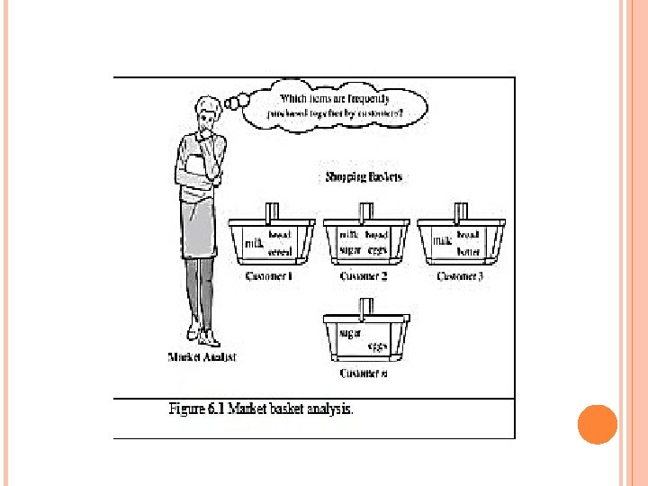
M ARKET BASKET ANALYSIS Frequent item set mining leads to the discovery of associations and correlations Items associated in large transactional or relational data sets. Discovery of interesting correlationships among huge amounts of business transaction records It help us in business decision-making processes such as catalog design, cross-marketing, and customer shopping behavior analysis. Items that are frequently purchased together can be placed in proximity to further encourage the combined sale of such items. For ex. who purchase computers also tend to buy antivirus software at the same time

WH Y I S F R E Q. P A TT E R N M I N G I M P O R T A N T ? Discloses an intrinsic and important property of data sets Forms the foundation for many essential data mining tasks Association, correlation, and causality analysis Sequential, structural (e. g. , sub-graph) patterns Pattern analysis in spatiotemporal, multimedia, time-series, and stream data Classification: associative classification Cluster analysis: frequent pattern-based clustering Data warehousing: iceberg cube and cube-gradient Semantic data compression: fascicles Broad applications

B A S I C C O N C E P T S : F R E Q U E N T P A TTE R N S AND ASSO CIATION R U L E S Transaction-id Items bought Itemset X = {x 1, … , x k } 10 A, B, D 20 A, C, D F ind all the rules X Y with minimum support and confidence 30 A, D, E 40 B, E, F 50 B, C, D, E, F Customer buys both Customer buys bread Customer buys milk support, s, probability that a transaction contains X Y confidence, c, conditional probability that a transaction having X also contains Y Let sup m in = 50%, confm in = 50% F req. Pat. : {A: 3, B: 3, D: 4, E: 3, A D : 3} Association rules: A D (60%, 100%) D A (60%, 75%)

FREQUENT ITEMSETS, ASSOCIATION RULES CLOSED ITEMSETS, AND I={ I 1, I 2, I 3…. I m } be an itemset. Let D , is a set of database transactions where each transaction T is a nonempty itemset called TID The rule A→B holds in the transaction set D with supports, where s is the percentage of transactions in D that contain A ᴜ B (i. e. , the union of sets A and B say, or, both A and B ). support(A→B ) = P(A ᴜ B)

The rule A → B has confidence c in the transaction set D , where c is the percentage of transactions in D containing A that also contain B. This is taken to be the conditional probability P(B| A) Confidence (A → B) = P(B| A)

A long itemset will contain a combinatorial number of shorter, frequent sub-itemsets. For example, a frequent itemset of length 100, such as contains frequent 1 -itemsets: Frequent 2 -itemsets: and so on. The total number of frequent itemsets that it contains

We introduce the concepts of closed frequent itemset and maximal frequent itemset. An itemset X is closed in a data set D if there exists no proper super-itemset Y 1 such that Y has the same support count as X in D. An itemset X is a closed frequent itemset in set D if X is both closed and frequent in D. An itemset X is a maximal frequent itemset (or max-itemset) in a data set D if X is frequent, and there exists no super-itemset Y such that and y is frequent in D

CLOSED AND MAXIMAL FREQUENT ITEMSETS be the set of closed frequent itemsets for a data set D satisfying a minimum support threshold, be the set of maximal frequent itemsets for D satisfying contains complete information regarding its corresponding frequent itemsets. only the support of the maximal itemsets. It does not contain the complete support information regarding its corresponding frequent itemsets

A transaction database has only two transactions M inimum support count threshold be two closed frequent itemsets and their support counts One maximal frequent itemset C a nnot include as a maximal frequent itemset because it has a frequent superset

C LOSED P ATTERNS AND M A X -P ATTE R N S A long pattern contains a combinatorial number of subpatterns, e. g. , {a 1, … , a 100} contains (100 1) + (100 2) + … + (110000) = 2100 – 1 = 1. 27*1030 sub-patterns! Solution: M i ne closed patterns and max-patterns instead An itemset X is closed if X is frequent and there exists no super-pattern Y כ X , with the same support as X (proposed by Pasquier, et al. @ I C D T ’ 99) An itemset X is a max-pattern if X is frequent and there exists no frequent super-pattern Y כ X (proposed by Bayardo @ S I G M O D ’ 98) Closed pattern is a lossless compression of freq. patterns Reducing the # of patterns and rules

C LOSED P ATTERNS M in_sup = 1. What is the set of closed itemset? <a 1, … , a 100>: 1 < a 1, … , a 50>: 2 What is the set of max-pattern? M A X -P ATTE R N S E xercise. D B = {<a 1, … , a 100>, < a 1, … , a 50>} AND <a 1, … , a 100>: 1 What is the set of all patterns? !!

S CALABLE M ETHODS P A TT E R N S FOR MINING F R EQUENT The downward closure property of frequent patterns Any subset of a frequent itemset must be frequent If {bread, butter, milk} is frequent, so is {bread, butter} i. e. , every transaction having {bread, butter, milk} also contains {bread, butter} Scalable mining methods: Three major approaches Apriori (Agrawal & Srikant@VLDB’ 94) Freq. pattern growth (FPgrowth—Han, Pei & Yin @SIGMOD’ 00) Vertical data format approach (Charm—Zaki & Hsiao @SDM’ 02)

A P R I O R I : A C A N D ID A T E G E N E R A T IO N -A N D -T E S T APPROAC H Apriori pruning principle: If there is any itemset which is infrequent, its superset should not be generated/tested! (Agrawal & Srikant @VLDB’ 94, Mannila, et al. @ KDD’ 94) Method: Initially, scan D B once to get frequent 1 -itemset Generate length (k+1) candidate itemsets from length k frequent itemsets Test the candidates against D B Terminate when no frequent or candidate set can be generated

All nonempty subsets of a frequent itemset must also be frequent. The Apriori property is based on the following observation. If an itemset I does not satisfy the minimum support threshold, min_sup, then I is not frequent If an item A is added to the itemset I, then the resulting itemset (i. e. , ) cannot occur more frequently than I. i. e.

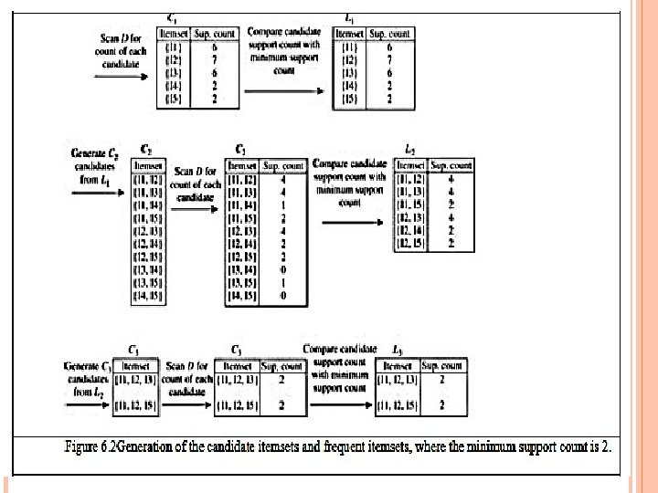
T H E A P R I O R I A L G O R I T H M —A N E X A M P L E Database TDB Tid Items 10 A, C, D 20 B, C, E 30 A, B, C, E 40 B, E S up min = 2 Itemset {A, C} {B, E} {C, E} sup {A} 2 {B} 3 {C} 3 {D} 1 {E} 3 C 1 1 st scan C 2 L 2 Itemset sup 2 2 3 2 Itemset {A, B} {A, C} {A, E} {B, C} {B, E} {C, E} sup 1 2 3 2 Itemset sup {A} 2 {B} 3 {C} 3 {E} 3 L 1 C 2 2 nd scan Itemset {A, B} {A, C} {A, E} {B, C} {B, E} {C, E} C 3 Itemset {B, C, E} 3 rd scan L 3 Itemset sup {B, C, E} 2

T H E A P R I O R I A L G O R IT H M Pseudo-code: C k : C andidate itemset of size k L k : frequent itemset of size k L 1 = {frequent items}; for (k = 1; L k != ; k++) do begin C k+1 = candidates generated from L k ; for each transaction t in database do increment the count of all candidates in C k+ 1 that are contained in t L k+1 = candidates in C k+1 with min_support end return k L k ;

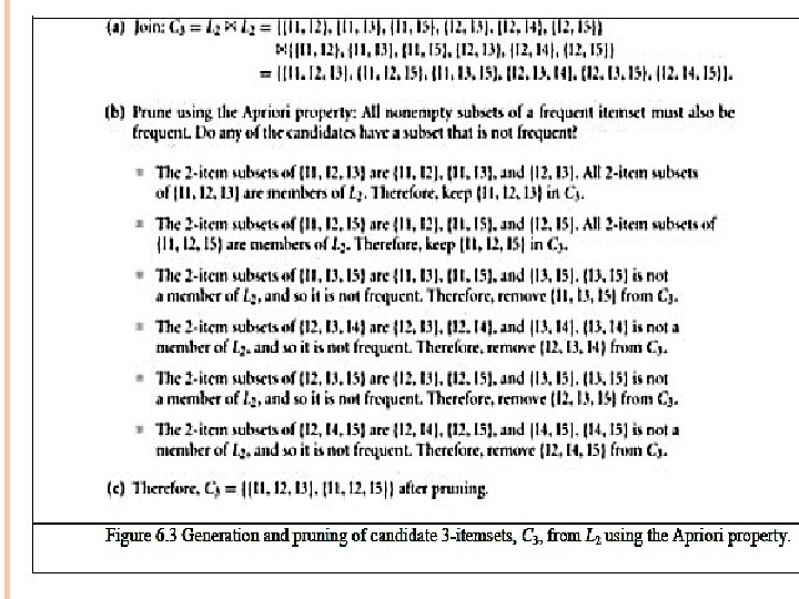
IMPORTANT D ETAILS OF APRIO RI How to generate candidates? Step 1: self-joining L k Step 2: pruning How to count supports of candidates? E xample of C a ndidate-generation L 3 ={abc, abd, ace, bcd} Self-joining: L 3 * L 3 abcd from abc and abd acde from acd and ace Pruning: acde is removed because ade is not in L 3 C 4 ={abcd}

H OW TO G E N E R A T E C A N D ID A T E S ? Suppose the items in L k-1 are listed in an order Step 1: self-joining L k-1 insert into C k select p. item 1, p. item 2, … , p. item k -1, q. item k -1 from L k -1 p, L k -1 q where p. item 1=q. item 1, … , p. item k -2=q. item k -2, p. item k -1 < q. item k -1 Step 2: pruning forall itemsets c in C k do forall (k-1)-subsets s of c do if (s is not in L k -1 ) then delete c from C k

C HALLENGES OF F R E Q U E N T P A TT E R N M I N G Challenges Multiple scans of transaction database Huge number of candidates Tedious workload of support counting for candidates Improving Apriori: general ideas Reduce passes of transaction database scans Shrink number of candidates F acilitate support counting of candidates

F U RTHER IMPROVE M ENT OF THE APRIORI M ETHOD Major computational challenges Multiple scans of transaction database Huge number of candidates Tedious workload of support counting candidates Improving Apriori: general ideas Reduce passes of transaction database scans Shrink number of candidates F acilitate support counting of candidates for

P ARTITION : S C A N D ATA B A S E O N L Y T W I C E Any itemset that is potentially frequent in D B must be frequent in at least one of the partitions of D B Scan 1: partition database and find local frequent patterns Scan 2: consolidate global frequent patterns A. S avasere, E. Om iecinski and S. Navathe, VLDB’ 95 DB 1 sup 1(i) < σDB 1 + DB 2 sup 2(i) < σDB 2 + + DBk supk(i) < σDBk = DB sup(i) < σDB

DHP: R E D U C E C A N D ID A T E S N UMBER OF A k-itemset whose corresponding hashing bucket count is below C a ndidates: a, b, c, d, e Hash entries {ab, ad, ae} {bd, be, de} … count itemsets 35 {ab, ad, ae} 88 {bd, be, de} . . . the threshold cannot be frequent 102 . . . THE {yz, qs, wt} H ash Table Frequent 1 -itemset: a, b, d, e ab is not a candidate 2 -itemset if the sum of count of {ab, ad, ae} is below support threshold J. Park, M. Chen, and P. Y u. An effective hash-based algorithm for mining association rules. SIGMOD’ 95

S AMPLIN G FOR F R E Q U E N T P A T T ER N S Select a sample of original database, mine frequent patterns within sample using Apriori Scan database once to verify frequent itemsets found in sample, only borders of closure of frequent patterns are checked E xample: check abcd instead of ab, ac, … , etc. Scan database again to find missed frequent patterns H. Toivonen. Sampling large databases for association rules. In VLDB’ 96

DIC: R E D U C E N U M B E R OF ABCD AB AC BC AD BD CD Once both A and D are determined frequent, the counting of A D begins Once all length-2 subsets of B C D are determined frequent, the counting of B C D begins Transactions A B C D Apriori {} Itemset lattice S. Brin R. M otwani, J. U llman, and S. Tsur. Dynamic itemset counting and implication rules for market basket data. In SIGMOD’ 97 1 -itemsets 2 -itemsets … 1 -itemsets 2 -items DIC 3 -items 33 ABC ABD ACD BCD SCANS

P A T T ER N -G R O WTH A P P R O A C H : M I N G F R E Q U E N T P A T T E R N S W IT H O U T C A N D I D A T E G E N E R A T I O N Bottlenecks of the Apriori approach Breadth-first (i. e. , level-wise) search Candidate generation and test 34 Often generates a huge number of candidates The F PGrowth Approach (J. Han, J. Pei, and Y. Y in, S I G M O D ’ 00) Depth-first search Avoid explicit candidate generation Major philosophy: Grow long patterns from short ones using local frequent items only “abc” is a frequent pattern Get all transactions having “abc”, i. e. , project D B on abc: D B | a b c “d” is a local frequent item in D B | a b c abcd is a frequent pattern

C O N S T R U C T F P -T R E E D ATABA S E T R AN S A C T I O N Items bought (ordered) frequent items {f, a, c, d, g, i, m, p} {f, c, a, m, p} {a, b, c, f, l, m, o} {f, c, a, b, m} min_support = 3 {b, f, h, j, o, w} {f, b} {b, c, k, s, p} {c, b, p} {a, f, c, e, l, p, m, n} {f, c, a, m, p} {} Header Table 1. Scan DB once, find f: 4 c: 1 Item frequency head frequent 1 -itemset (single 4 f item pattern) c: 3 b: 1 4 c 3 2. Sort frequent items in a 3 b frequency descending p: 1 a: 3 3 m order, f-list 3 p m: 2 b: 1 3. Scan DB again, construct FP-tree p: 2 m: 1 F-list = f-c-a-b-m-p 35 TID 100 200 300 400 500 FROM A

P ARTITION P ATT E R N S AND D ATA B A S E S Frequent patterns can be partitioned into subsets according to f-list Completeness and non-redundency 36 F -list = f-c-a-b-m-p Patterns containing p Patterns having m but no p … Patterns having c but no a nor b, m , p Pattern f

F IND P A T T E R N S H A V I N G P F R O M P-C O N D I T I O N A L D ATABA S E 37 Starting at the frequent item header table in the F P -tree Traverse the F P -tree by following the link of each frequent item p Accumulate all of transformed prefix paths of item p to form p’s conditional pattern base {} Header Table Item frequency head f 4 c 4 a 3 b 3 m 3 p 3 c: 1 f: 4 c: 3 b: 1 a: 3 p: 1 m: 2 b: 1 p: 2 m: 1 Conditional pattern bases item c cond. pattern base a b fc: 3 fca: 1, f: 1, c: 1 m fca: 2, fcab: 1 p fcam: 2, cb: 1 f: 3

F R O M C O N D I T IO N A L P ATTE R N -B A S E S TO C ONDITIONAL F P - TREES Header Table Item frequency head 4 f 4 c 3 a 3 b 3 m 3 p {} f: 4 c: 3 c: 1 b: 1 a: 3 b: 1 p: 1 m: 2 b: 1 p: 2 m: 1 38 For each pattern-base Accumulate the count for each item in the base Construct the F P -tree for the frequent items of the pattern base m-conditional pattern base: fca: 2, fcab: 1 All frequent patterns relate to m {} m, f: 3 fm, cm, am, fcm, fam, c: 3 fcam a: 3 m-conditional FP-tree

R E C U R S I O N : M I N IN G E A C H C O N D I T I O N A L F P TREE {} {} Cond. pattern base of “am”: (fc: 3) a: 3 39 c: 3 f: 3 am-conditional FP-tree Cond. pattern base of “cm”: (f: 3) {} f: 3 m-conditional FP-tree cm-conditional FP-tree {} Cond. pattern base of “cam”: (f: 3) f: 3 cam-conditional FP-tree

A S P E C I A L C A S E : S I N G L E P R E F IX P A T H IN FP- TREE Suppose a (conditional) F P -tree T has a shared single prefix-path P Mining can be decomposed into two parts {} a 1: n 1 a 2: n 2 Reduction of the single prefix path into one node Concatenation of the mining results of the two parts a 3: n 3 b 1: m 1 C 2: k 2 40 r 1 {} C 1: k 1 C 3: k 3 r 1 = a 1: n 1 a 2: n 2 a 3: n 3 + C 1: k 1 b 1: m 1 C 2 : k 2 C 3 : k 3

BENEFITS F P -T R E E S T R U C T U R E Completeness Preserve complete information for frequent pattern mining Never break a long pattern of any transaction 41 OF THE Compactness Reduce irrelevant info—infrequent items are gone Items in frequency descending order: the more frequently occurring, the more likely to be shared Never be larger than the original database (not count node-links and the count field)

T H E F R E Q U E N T P A T T E R N G R O W T H M I N IN G M ETHOD Idea: F requent pattern growth Recursively grow frequent patterns by pattern and database partition Method For each frequent item, construct its conditional pattern-base, and then its conditional F P -tree Repeat the process on each newly created conditional F P -tree Until the resulting F P -tree is empty, or it contains only one path—single path will generate all the combinations of its sub-paths, each of which is a frequent pattern 42

S C A L IN G F P -G R O W T H BY D ATABA S E P R O J E C T IO N What about if F P -tree cannot fit in memory? D B projection First partition a database into a set of projected D B s Then construct and mine F P-tree for each projected D B Parallel projection vs. partition projection techniques Parallel projection Project the D B in parallel for each frequent item Parallel projection is space costly All the partitions can be processed in parallel Partition projection Partition the D B based on the ordered frequent items Passing the unprocessed parts to the subsequent partitions 43

P ART ITION -B A S E D P R O J E C T IO N Partition projection saves it Tran. DB fcamp fcabm fb cbp fcamp 44 Parallel projection needs a lot of disk space p-proj DB m-proj DB b-proj DB a-proj DB c-proj DB fcam cb fcam fcab fca am-proj DB f cb … fc … cm-proj DB fc fc f f f … … f-proj DB …

M U L T I P L E -L E V E L A S S O C I A T IO N R U L E S Food Items often form hierarchy. Items at the lower level are expected to have lower support. Rules regarding itemsets at appropriate levels could be quite useful. Transaction database can be encoded based on dimensions and levels We can explore shared multi-level mining bread milk skim Fraser TID T 1 T 2 T 3 T 4 T 5 2% wheat white Sunset Items {111, 121, 211, 221} {111, 222, 323} {112, 122, 221, 411} {111, 122, 211, 221, 413}

M I N IN G M U L T I -L E V E L A S S O C I A T IO N S A top_down, progressive deepening approach: First find high-level strong rules: milk bread [20%, 60%]. Then find their lower-level “weaker” rules: 2% milk wheat bread [6%, 50%]. Variations at mining multiplelevel association rules. Level-crossed association rules: 2% milk Wonder wheat bread Association rules with multiple, alternative hierarchies:

M U L T I -L E V E L A S S O C I A T I O N : U N I F O R M S UPPORT VS. REDUCED S UPPORT Uniform Support: the same minimum support for all levels + One minimum support threshold. No need to examine itemsets containing any item whose ancestors do not have minimum support. – Lower level items do not occur as frequently. If support threshold too high miss low level associations too low generate too many high level associations Reduced Support: reduced minimum support at lower levels There are 4 search strategies: Level-by-level independent Level-cross filtering by k-itemset Level-cross filtering by single item Controlled level-cross filtering by single item

U NIFORM S UPPORT Multi-level mining with uniform support Level 1 min_sup = 5% Level 2 min_sup = 5% Milk [support = 10%] 2% Milk Skim Milk [support = 6%] [support = 4%]

RE D U C E D S UPPORT Multi-level mining with reduced support Milk Level 1 min_sup = 5% Level 2 min_sup = 3% [support = 10%] 2% Milk Skim Milk [support = 6%] [support = 4%]

M U L T I -L E V E L A S S O C I A T I O N : R E D U N D A N C Y F I L T E R IN G Some rules may be redundant due to “ancestor” relationships between items. Example milk wheat bread [support = 8%, confidence = 70%] 2% milk wheat bread [support = 2%, confidence = 72%] We say the first rule is an ancestor of the second rule. A rule is redundant if its support is close to the “expected” value, based on the rule’s ancestor.

M U L T I -L E V E L M I N G : P R O G R E S S I V E DEEPENING A top-down, progressive deepening approach: First mine high-level frequent items: milk (15%), bread (10%) Then mine their lower-level “weaker” frequent itemsets: 2% milk (5%), wheat bread (4%) Different min_support threshold across multi-levels lead to different algorithms: If adopting the same min_support across multilevels then loss t if any of t’s ancestors is infrequent. If adopting reduced min_support at lower levels then examine only those descendents whose ancestor’s support is frequent/non-negligible.

PROGRESSIVE REFINEMENT D ATA M I N G Q U A L I T Y Why progressive refinement? M ining operator can be expensive or cheap, fine or rough Trade speed with quality: step-by-step refinement. Superset coverage property: OF Preserve all the positive answers—allow a positive false test but not a false negative test. Two- or multi-step mining: First apply rough/cheap operator (superset coverage) Then apply expensive algorithm on a substantially reduced candidate set (Koperski & Han, S S D’ 95).

C O N S T R A INT -B A S E D M I N IN G Interactive, of data? exploratory mining giga-bytes Could it be real? — Making good use of constraints! What kinds of constraints can be used in mining? Knowledge type constraint: classification, association, etc. Data constraint: S Q L -like queries Dimension/level constraints: in relevance to region, price, brand, customer category. Rule constraints Find product pairs sold together in V ancouver in Dec. ’ 98. small sales (price < $10) triggers big sales (sum > $200). Interestingness constraints: strong rules (min_support 3%, min_confidence 60%).

RU L E C ONSTRAINTS Two ASSOCIATION M INING kind of rule constraints: Rule form constraints: meta-rule guided mining. IN P(x, y) ^ Q (x, w) takes(x, “database systems”). Rule (content) constraint: constraint-based query optimization (Ng, et al. , S I G M O D’ 98). sum(LHS) < 100 ^ min(LHS) > 20 ^ count(LHS) > 3 ^ sum(RHS) > 1000 1 -variable vs. 2 -variable et al. S I G M O D ’ 99): constraints (Lakshmanan, 1 -var: A constraint confining only one side (L/R) of the rule, e. g. , as shown above. 2 -var: A constraint confining both sides (L and R). sum(LHS) < min(RHS) ^ max(RHS) < 5* sum(LHS)

C O N S T R A I N -B A S E D A S S O C I A T IO N Q U E R Y Database: (1) trans (TID, Itemset ), (2) item. Info (Item , Type, Price) A constrained asso. query (CAQ) is in the form of {(S 1, S 2 )| C }, where C is a set of constraints on S 1, S 2 including frequency constraint A classification of (single-variable) constraints: C lass constraint: S A. e. g. S Item Domain constraint: S v, { , , , }. e. g. S. P r ice < 100 v S , is or . e. g. snacks S. T ype V S , or S V , { , , } e. g. {snacks, sodas } S. T ype Aggregation constraint: agg(S) v, where agg is in {min, max, sum , count, avg}, and { , , , }. e. g. count(S 1. Type) 1 , avg(S 2. Price) 100

C O N STRA I N E D A S S O C I A T IO N Q U E R Y O PTIMIZA T I O N P R O B LE M G iven a C A Q = { (S 1, S 2) | C }, the algorithm should be : sound: It only finds frequent sets that satisfy the given constraints C complete: All frequent sets satisfy the given constraints C are found A naïve solution: Apply Apriori for finding all frequent sets, and then to test them for constraint satisfaction one by one. Our approach: Comprehensive analysis of the properties of constraints and try to push them as deeply as possible inside the frequent set computation.

A N T I -M O N O T O N E C O N STRA I N T S AND M ONOTONE A constraint C a is anti-monotone iff. for any pattern S not satisfying C a , none of the superpatterns of S can satisfy C a A constraint C m is monotone iff. for any pattern S satisfying C m , every super-pattern of S also satisfies it

S U C C I N C T C O N S T R A INT A subset of item I s is a succinct set, if it can be expressed as p(I) for some selection predicate p, where is a selection operator S P 2 I is a succinct power set, if there is a fixed number of succinct set I 1, … , I k I, s. t. S P can be expressed in terms of the strict power sets of I 1, … , I k using union and minus A constraint C s is succinct provided SAT (I) is a succinct

C O N V E R T I B L E C O N S T R A INT Suppose all items in patterns are listed in a total order R A constraint C is convertible antimonotone iff a pattern S satisfying the constraint implies that each suffix of S w. r. t. R also satisfies C A constraint C is convertible monotone iff a pattern S satisfying the constraint implies that each pattern of which S is a suffix w. r. t. R also satisfies C

R E L A T IO N S H IP S A M O N G C A T EG O R I E S C O N STRA I N T S Succinctness Anti-monotonicity Monotonicity Convertible constraints Inconvertible constraints OF

P R O PE R T Y O F C O N S T R A IN TS : A N T I -M O N O T O N E Anti-monotonicity: If a set S violates the constraint, any superset of S violates the constraint. E xamples: sum(S. Price) v is anti-monotone sum(S. Price) v is not anti-monotone sum(S. Price) = v is partly anti-monotone Application: Push “sum(S. price) 1000” deeply into iterative frequent set computation.

C HARACTERIZATION OF A N T I -M O N O T O N I C I T Y C O N S T R A I N T S S v, { , , } v S S V S V min(S) v max(S) v count(S) v sum(S) v avg(S) v, { , , } (frequent constraint) yes no no yes partly yes no partly convertible (yes)

E X A M P L E O F C O N V E R T IB L E C O N S T R A INT S : A V G (S) V Let R be the value descending order over the set of items E. g. I={9, 8, 6, 4, 3, 1} Avg(S) v is convertible monotone w. r. t. R If S is a suffix of S 1, avg(S 1) avg(S) {8, 4, 3} is a suffix of {9, 8, 4, 3} avg({9, 8, 4, 3})=6 avg({8, 4, 3})=5 If S satisfies avg(S) v, so does S 1 {8, 4, 3} satisfies constraint avg(S) 4, so does {9, 8, 4, 3}

P R O P E R T Y O F C O N S T R A INT S : SUCCINCTNESS Succinctness: For any set S 1 and S 2 satisfying C , S 1 S 2 satisfies C Given A 1 is the sets of size 1 satisfying C , then any set S satisfying C are based on A 1 , i. e. , it contains a subset belongs to A 1 , Example : sum(S. Price ) v is not succinct min(S. Price ) v is succinct Optimization: If C is succinct, then C is pre-counting prunable. The satisfaction of the constraint alone is not affected by the iterative support counting.

C H A R A C T E R IZATIO N SUCCINCTNESS OF S v, { , , } v S S V S V min(S) v max(S) v count(S) v sum(S) v avg(S) v, { , , } (frequent constraint) C O N STRA I N T S Yes yes yes yes weakly no no (no) BY