Deep Generative Models An Overview Yidong Chai 1

Deep Generative Models: An Overview Yidong Chai 1, 2, Weifeng Li 1, 3, Hsinchun Chen 1 1 Artificial Intelligence Laboratory, The University of Arizona 2 Tsinghua University 3 University of Georgia 1

Acknowledgements • Many of the pictures, results, and other materials are taken from: • • Aaron Courville, University of Montreal Diederik P. Kingma, University of Amsterdam/Open. AI/Google. Brain Eric Xing, Carnegie Mellon University/Petuum Inc. Geoffrey Hinton, Google & University of Toronto Ian J. Goodfellow, Google Brain Stefano Eron, Stanford University Yoshua Bengio, Universite de Montreal 2

Outline • Introduction • Traditional Generative Models • Deep Generative Models • Example Applications • Deep Belief Networks • Variational Autoencoder • Technical novelties • Implementation • Generative Adversarial Networks • Technical novelties • Implementation • Research Example: Motion Sensor-Based Fall Detection and Prediction • Conclusions • Appendix 3

Outline • Introduction • Traditional Generative Models • Deep Generative Models • Example Applications • Deep Belief Networks • Variational Autoencoder • Technical novelties • Implementation • Generative Adversarial Networks • Technical novelties • Implementation • Research Example: Motion Sensor-Based Fall Detection and Prediction • Conclusions • Appendix 4

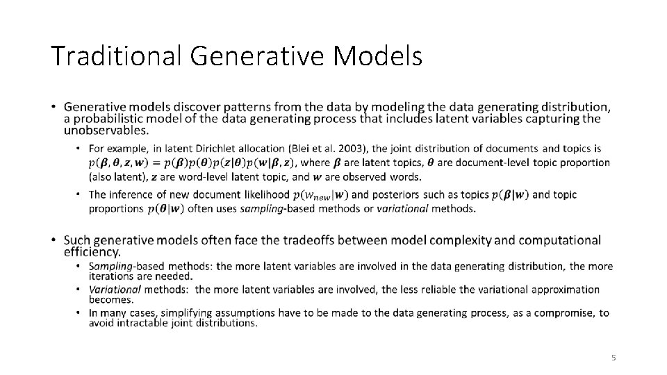
Traditional Generative Models • 5

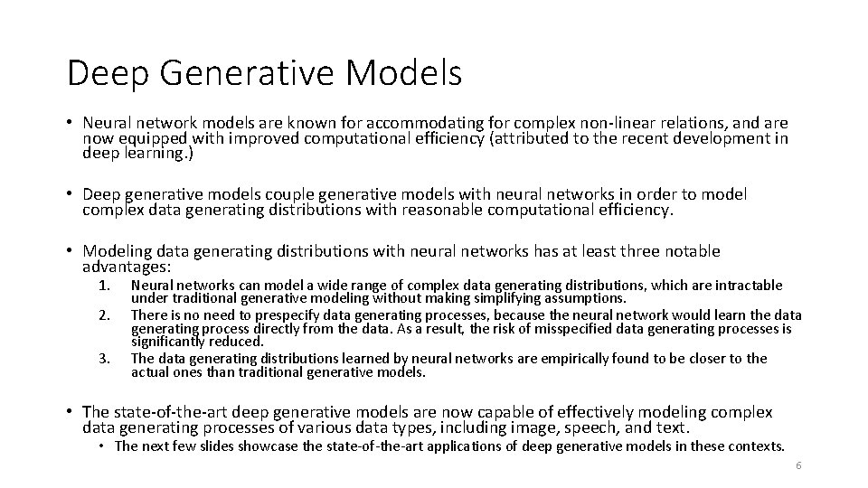
Deep Generative Models • Neural network models are known for accommodating for complex non-linear relations, and are now equipped with improved computational efficiency (attributed to the recent development in deep learning. ) • Deep generative models couple generative models with neural networks in order to model complex data generating distributions with reasonable computational efficiency. • Modeling data generating distributions with neural networks has at least three notable advantages: 1. 2. 3. Neural networks can model a wide range of complex data generating distributions, which are intractable under traditional generative modeling without making simplifying assumptions. There is no need to prespecify data generating processes, because the neural network would learn the data generating process directly from the data. As a result, the risk of misspecified data generating processes is significantly reduced. The data generating distributions learned by neural networks are empirically found to be closer to the actual ones than traditional generative models. • The state-of-the-art deep generative models are now capable of effectively modeling complex data generating processes of various data types, including image, speech, and text. • The next few slides showcase the state-of-the-art applications of deep generative models in these contexts. 6

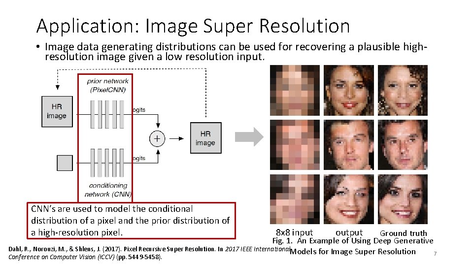
Application: Image Super Resolution • Image data generating distributions can be used for recovering a plausible highresolution image given a low resolution input. CNN’s are used to model the conditional distribution of a pixel and the prior distribution of a high-resolution pixel. 8 x 8 input output Ground truth Fig. 1. An Example of Using Deep Generative Dahl, R. , Norouzi, M. , & Shlens, J. (2017). Pixel Recursive Super Resolution. In 2017 IEEE International. Models for Image Super Resolution 7 Conference on Computer Vision (ICCV) (pp. 5449 -5458).

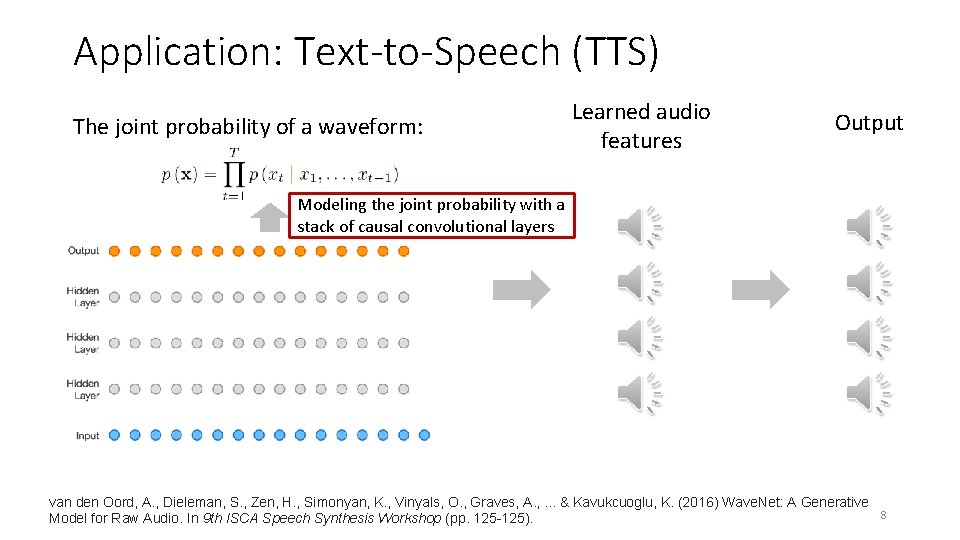
Application: Text-to-Speech (TTS) The joint probability of a waveform: Learned audio features Output Modeling the joint probability with a stack of causal convolutional layers van den Oord, A. , Dieleman, S. , Zen, H. , Simonyan, K. , Vinyals, O. , Graves, A. , . . . & Kavukcuoglu, K. (2016) Wave. Net: A Generative 8 Model for Raw Audio. In 9 th ISCA Speech Synthesis Workshop (pp. 125 -125).

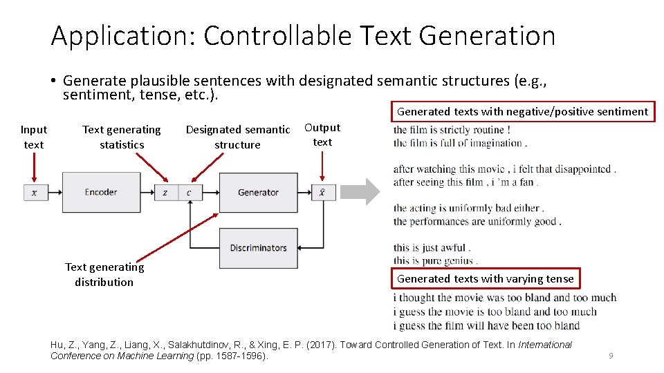
Application: Controllable Text Generation • Generate plausible sentences with designated semantic structures (e. g. , sentiment, tense, etc. ). Generated texts with negative/positive sentiment Input text Text generating statistics Text generating distribution Designated semantic Output text structure Generated texts with varying tense Hu, Z. , Yang, Z. , Liang, X. , Salakhutdinov, R. , & Xing, E. P. (2017). Toward Controlled Generation of Text. In International Conference on Machine Learning (pp. 1587 -1596). 9

Deep Generative Models • In this set of slides, we will introduce three most representative deep generative models: Deep Belief Networks, Variational Autoencoders, and Generative Adversarial Networks. • Deep Belief Networks (DBN) employ layer-wise generative modeling to initialize each layer and simultaneously capture multiple levels of data representation. • Started the recent deep learning renaissance • Hinton, G. E, Osindero, S. , and Teh, Y. W. (2006). A fast learning algorithm for deep belief nets. Neural Computation, 18: 1527 -1554. • Variational Autoncoder (VAE) is a variational algorithm that infers the statistical characteristics of latent variables using an autoencoder neural network architecture. • Kingma, D. P. , & Welling, M. (2014). Auto-Encoding Variational Bayes. In Proceedings of International Conference on Learning Representations (ICLR). • Generative Adversarial Networks (GAN) train two neural networks (a generative neural network and a discriminative neural network) contesting with each other in a zero-sum game framework. • Goodfellow, I. , Pouget-Abadie, J. , Mirza, M. , Xu, B. , Warde-Farley, D. , Ozair, S. , … Bengio, Y. (2014). Generative Adversarial Nets. In Advances in Neural Information Processing Systems 27 (pp. 2672– 2680). 10

Outline • Introduction • Traditional Generative Models • Deep Generative Models • Example Applications • Deep Belief Networks • Variational Autoencoder • Technical novelties • Implementation • Generative Adversarial Networks • Technical novelties • Implementation • Research Example: Motion Sensor-Based Fall Detection and Prediction • Conclusions • Appendix 11

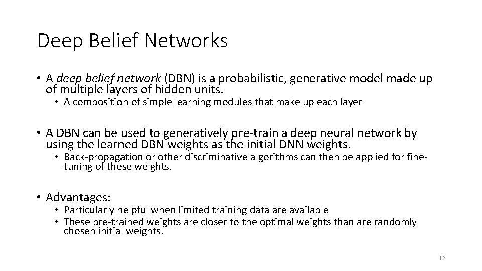
Deep Belief Networks • A deep belief network (DBN) is a probabilistic, generative model made up of multiple layers of hidden units. • A composition of simple learning modules that make up each layer • A DBN can be used to generatively pre-train a deep neural network by using the learned DBN weights as the initial DNN weights. • Back-propagation or other discriminative algorithms can then be applied for finetuning of these weights. • Advantages: • Particularly helpful when limited training data are available • These pre-trained weights are closer to the optimal weights than are randomly chosen initial weights. 12

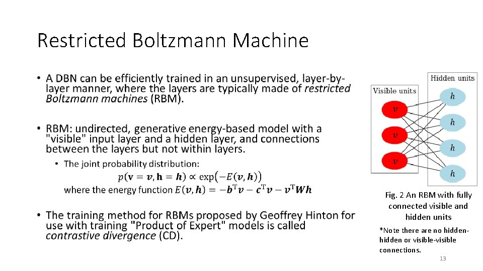
Restricted Boltzmann Machine • Fig. 2 An RBM with fully connected visible and hidden units *Note there are no hidden or visible-visible connections. 13

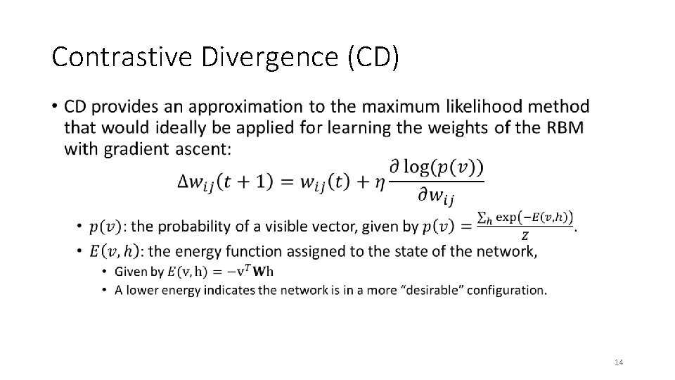
Contrastive Divergence (CD) • 14

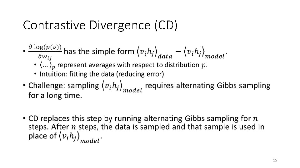
Contrastive Divergence (CD) • 15

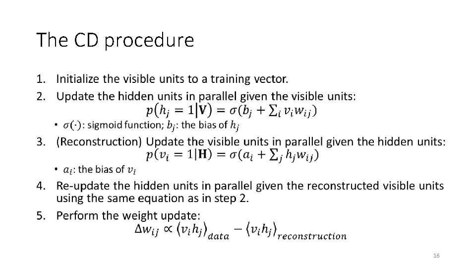
The CD procedure • 16

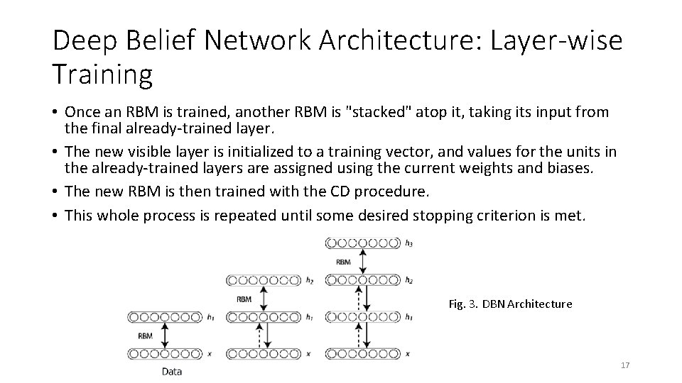
Deep Belief Network Architecture: Layer-wise Training • Once an RBM is trained, another RBM is "stacked" atop it, taking its input from the final already-trained layer. • The new visible layer is initialized to a training vector, and values for the units in the already-trained layers are assigned using the current weights and biases. • The new RBM is then trained with the CD procedure. • This whole process is repeated until some desired stopping criterion is met. Fig. 3. DBN Architecture 17

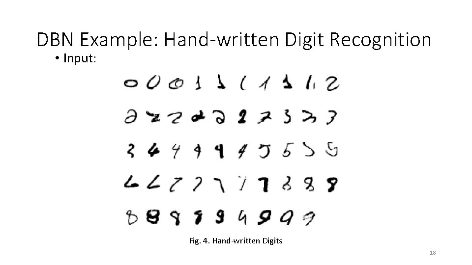
DBN Example: Hand-written Digit Recognition • Input: Fig. 4. Hand-written Digits 18

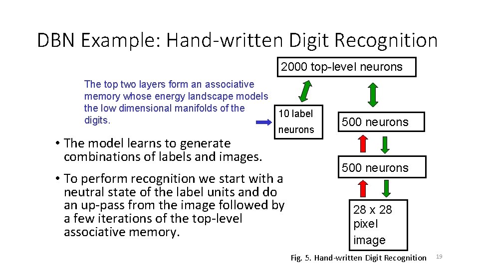
DBN Example: Hand-written Digit Recognition 2000 top-level neurons The top two layers form an associative memory whose energy landscape models the low dimensional manifolds of the 10 label digits. neurons • The model learns to generate combinations of labels and images. • To perform recognition we start with a neutral state of the label units and do an up-pass from the image followed by a few iterations of the top-level associative memory. 500 neurons 28 x 28 pixel image Fig. 5. Hand-written Digit Recognition 19

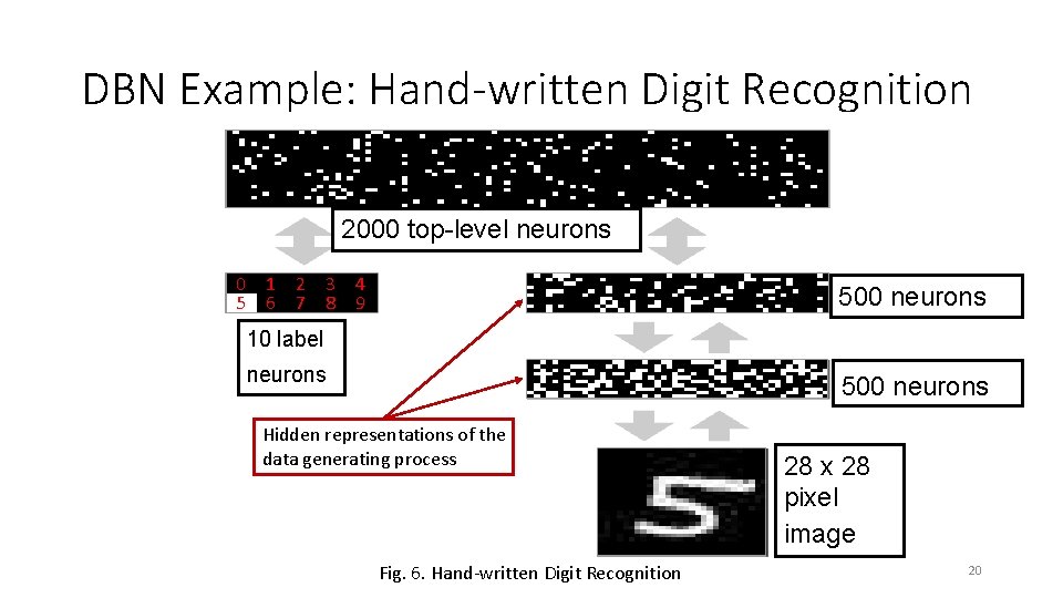
DBN Example: Hand-written Digit Recognition 2000 top-level neurons 0 5 1 6 2 7 3 8 4 9 500 neurons 10 label neurons 500 neurons Hidden representations of the data generating process Fig. 6. Hand-written Digit Recognition 28 x 28 pixel image 20

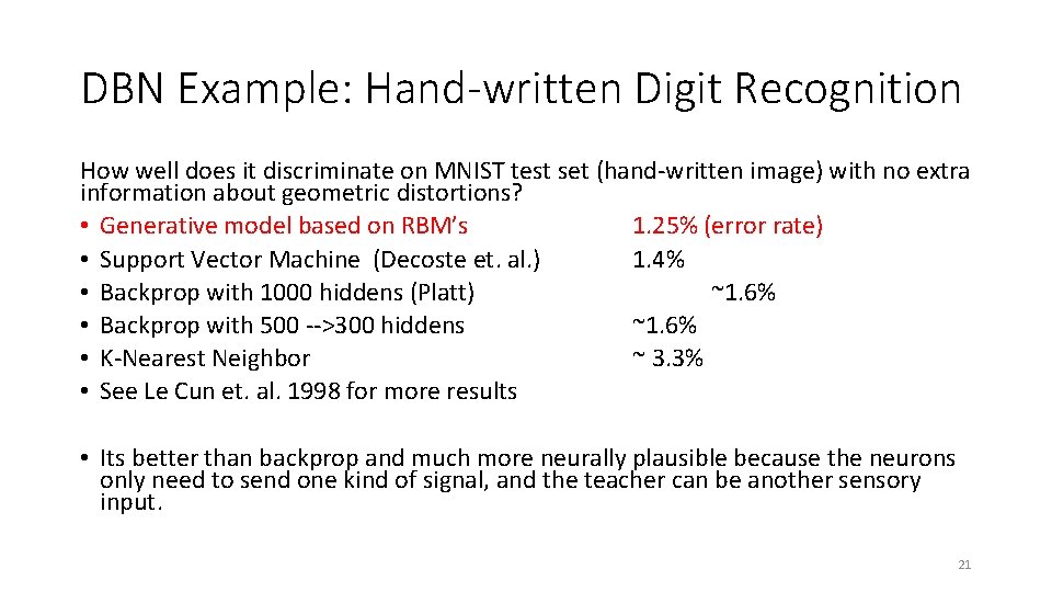
DBN Example: Hand-written Digit Recognition How well does it discriminate on MNIST test set (hand-written image) with no extra information about geometric distortions? • Generative model based on RBM’s 1. 25% (error rate) • Support Vector Machine (Decoste et. al. ) 1. 4% • Backprop with 1000 hiddens (Platt) ~1. 6% • Backprop with 500 -->300 hiddens ~1. 6% • K-Nearest Neighbor ~ 3. 3% • See Le Cun et. al. 1998 for more results • Its better than backprop and much more neurally plausible because the neurons only need to send one kind of signal, and the teacher can be another sensory input. 21

Outline • Introduction • Traditional Generative Models • Deep Generative Models • Example Applications • Deep Belief Networks • Variational Autoencoder • Technical novelties • Implementation • Generative Adversarial Networks • Technical novelties • Implementation • Research Example: Motion Sensor-Based Fall Detection and Prediction • Conclusions • Appendix 22

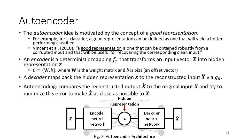
Autoencoder • Hidden Representation Encoder neural network z Decoder neural network Fig. 7. Autoencoder Architecture 23

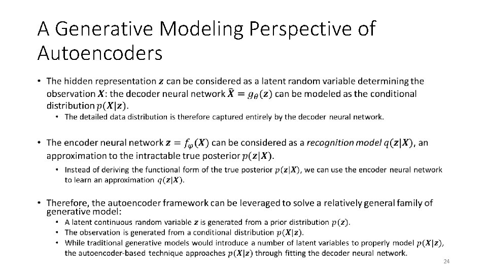
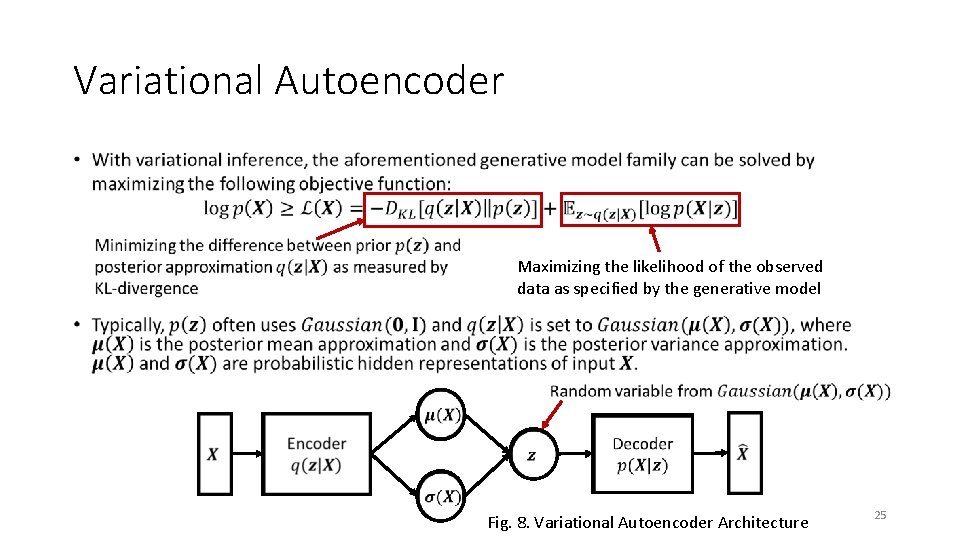
A Generative Modeling Perspective of Autoencoders • 24

Variational Autoencoder • Maximizing the likelihood of the observed data as specified by the generative model Fig. 8. Variational Autoencoder Architecture 25

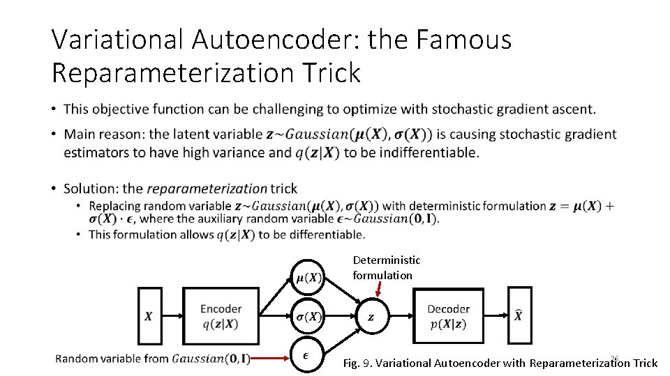
Variational Autoencoder: the Famous Reparameterization Trick • Deterministic formulation 26 Fig. 9. Variational Autoencoder with Reparameterization Trick

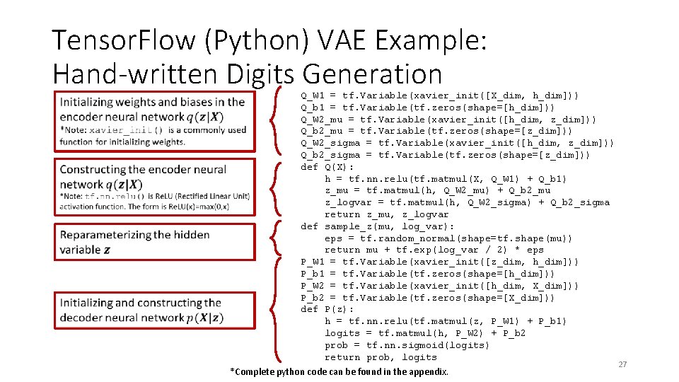
Tensor. Flow (Python) VAE Example: Hand-written Digits Generation Q_W 1 = tf. Variable(xavier_init([X_dim, h_dim])) Q_b 1 = tf. Variable(tf. zeros(shape=[h_dim])) Q_W 2_mu = tf. Variable(xavier_init([h_dim, z_dim])) Q_b 2_mu = tf. Variable(tf. zeros(shape=[z_dim])) Q_W 2_sigma = tf. Variable(xavier_init([h_dim, z_dim])) Q_b 2_sigma = tf. Variable(tf. zeros(shape=[z_dim])) def Q(X): h = tf. nn. relu(tf. matmul(X, Q_W 1) + Q_b 1) z_mu = tf. matmul(h, Q_W 2_mu) + Q_b 2_mu z_logvar = tf. matmul(h, Q_W 2_sigma) + Q_b 2_sigma return z_mu, z_logvar def sample_z(mu, log_var): eps = tf. random_normal(shape=tf. shape(mu)) return mu + tf. exp(log_var / 2) * eps P_W 1 = tf. Variable(xavier_init([z_dim, h_dim])) P_b 1 = tf. Variable(tf. zeros(shape=[h_dim])) P_W 2 = tf. Variable(xavier_init([h_dim, X_dim])) P_b 2 = tf. Variable(tf. zeros(shape=[X_dim])) def P(z): h = tf. nn. relu(tf. matmul(z, P_W 1) + P_b 1) logits = tf. matmul(h, P_W 2) + P_b 2 prob = tf. nn. sigmoid(logits) return prob, logits *Complete python code can be found in the appendix. 27

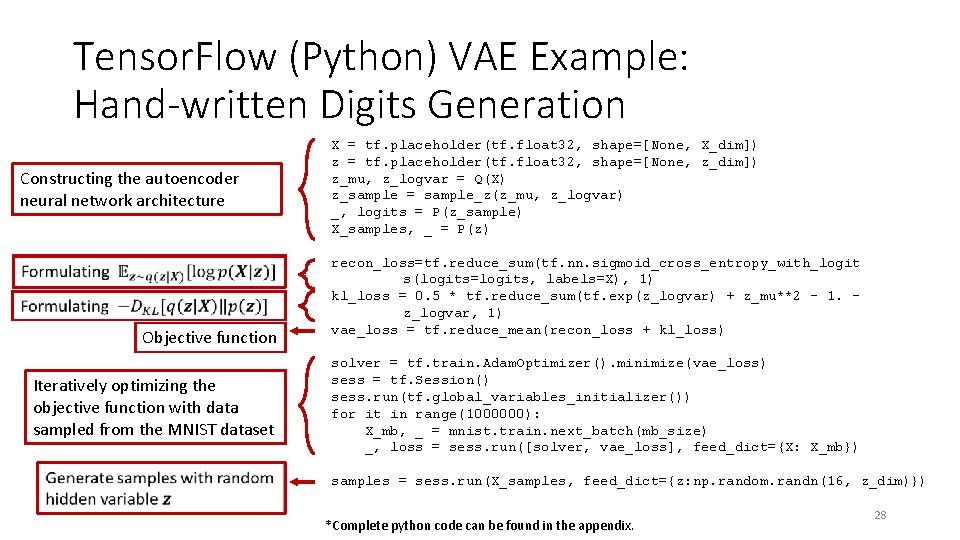
Tensor. Flow (Python) VAE Example: Hand-written Digits Generation Constructing the autoencoder neural network architecture Objective function Iteratively optimizing the objective function with data sampled from the MNIST dataset X = tf. placeholder(tf. float 32, shape=[None, X_dim]) z = tf. placeholder(tf. float 32, shape=[None, z_dim]) z_mu, z_logvar = Q(X) z_sample = sample_z(z_mu, z_logvar) _, logits = P(z_sample) X_samples, _ = P(z) recon_loss=tf. reduce_sum(tf. nn. sigmoid_cross_entropy_with_logit s(logits=logits, labels=X), 1) kl_loss = 0. 5 * tf. reduce_sum(tf. exp(z_logvar) + z_mu**2 - 1. z_logvar, 1) vae_loss = tf. reduce_mean(recon_loss + kl_loss) solver = tf. train. Adam. Optimizer(). minimize(vae_loss) sess = tf. Session() sess. run(tf. global_variables_initializer()) for it in range(1000000): X_mb, _ = mnist. train. next_batch(mb_size) _, loss = sess. run([solver, vae_loss], feed_dict={X: X_mb}) samples = sess. run(X_samples, feed_dict={z: np. random. randn(16, z_dim)}) *Complete python code can be found in the appendix. 28

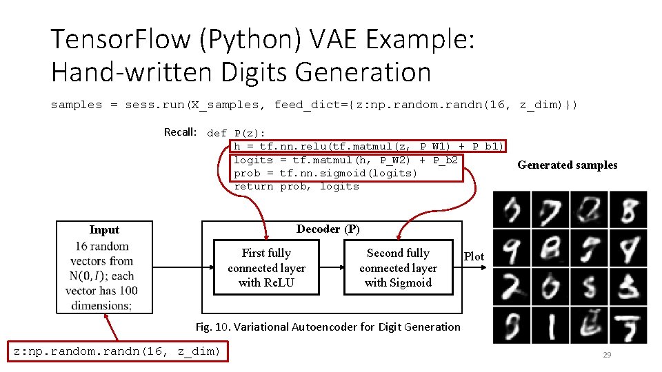
Tensor. Flow (Python) VAE Example: Hand-written Digits Generation samples = sess. run(X_samples, feed_dict={z: np. random. randn(16, z_dim)}) Recall: def P(z): h = tf. nn. relu(tf. matmul(z, P_W 1) + P_b 1) logits = tf. matmul(h, P_W 2) + P_b 2 prob = tf. nn. sigmoid(logits) return prob, logits Generated samples Decoder (P) Input First fully connected layer with Re. LU Second fully connected layer with Sigmoid Plot Fig. 10. Variational Autoencoder for Digit Generation z: np. random. randn(16, z_dim) 29

Outline • Introduction • Traditional Generative Models • Deep Generative Models • Example Applications • Deep Belief Networks • Variational Autoencoder • Technical novelties • Implementation • Generative Adversarial Networks • Technical novelties • Implementation • Research Example: Motion Sensor-Based Fall Detection and Prediction • Conclusions • Appendix 30

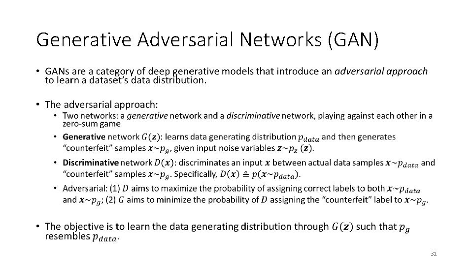
Generative Adversarial Networks (GAN) • 31

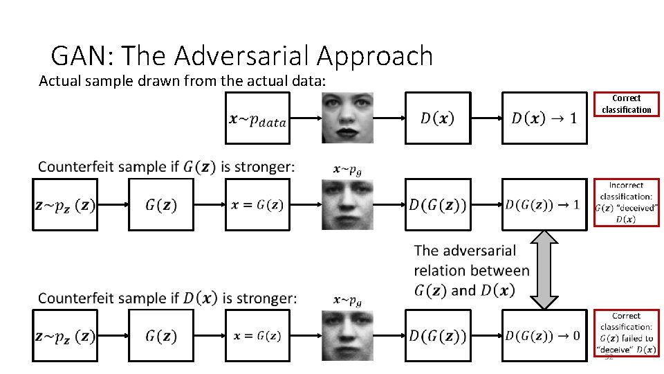
GAN: The Adversarial Approach Actual sample drawn from the actual data: Correct classification 32

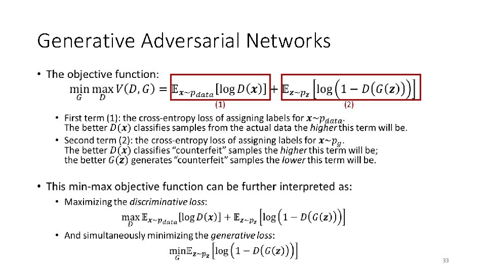
Generative Adversarial Networks • (1) (2) 33

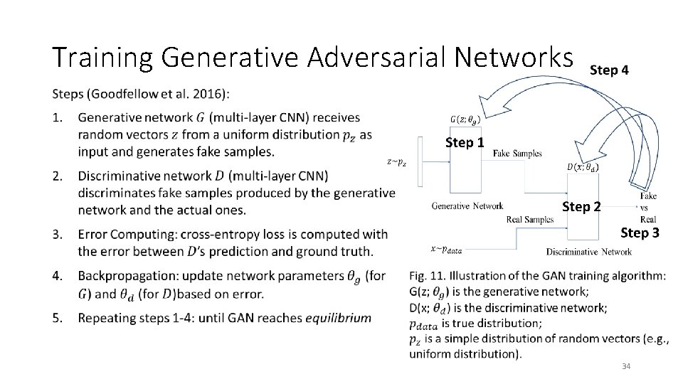
Training Generative Adversarial Networks • 34

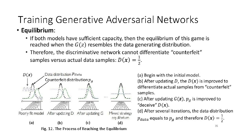
Training Generative Adversarial Networks • (c) (a) (b) (d) Fig. 12. The Process of Reaching the Equilibrium 35

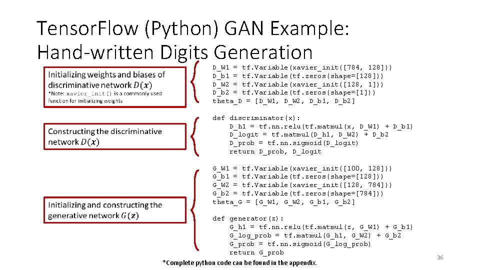
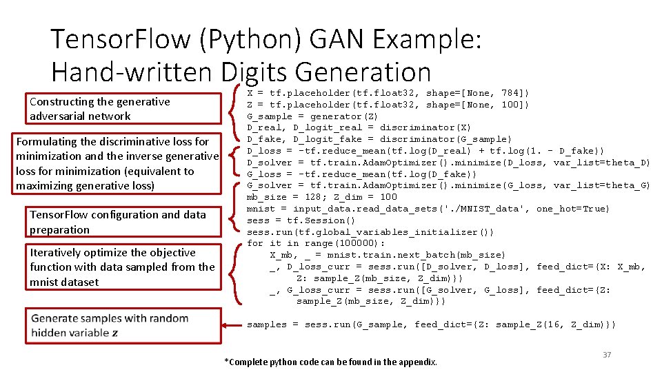
Tensor. Flow (Python) GAN Example: Hand-written Digits Generation D_W 1 = tf. Variable(xavier_init([784, 128])) D_b 1 = tf. Variable(tf. zeros(shape=[128])) D_W 2 = tf. Variable(xavier_init([128, 1])) D_b 2 = tf. Variable(tf. zeros(shape=[1])) theta_D = [D_W 1, D_W 2, D_b 1, D_b 2] def discriminator(x): D_h 1 = tf. nn. relu(tf. matmul(x, D_W 1) + D_b 1) D_logit = tf. matmul(D_h 1, D_W 2) + D_b 2 D_prob = tf. nn. sigmoid(D_logit) return D_prob, D_logit G_W 1 = tf. Variable(xavier_init([100, 128])) G_b 1 = tf. Variable(tf. zeros(shape=[128])) G_W 2 = tf. Variable(xavier_init([128, 784])) G_b 2 = tf. Variable(tf. zeros(shape=[784])) theta_G = [G_W 1, G_W 2, G_b 1, G_b 2] def generator(z): G_h 1 = tf. nn. relu(tf. matmul(z, G_W 1) + G_b 1) G_log_prob = tf. matmul(G_h 1, G_W 2) + G_b 2 G_prob = tf. nn. sigmoid(G_log_prob) return G_prob *Complete python code can be found in the appendix. 36

Tensor. Flow (Python) GAN Example: Hand-written Digits Generation Constructing the generative adversarial network Formulating the discriminative loss for minimization and the inverse generative loss for minimization (equivalent to maximizing generative loss) Tensor. Flow configuration and data preparation Iteratively optimize the objective function with data sampled from the mnist dataset X = tf. placeholder(tf. float 32, shape=[None, 784]) Z = tf. placeholder(tf. float 32, shape=[None, 100]) G_sample = generator(Z) D_real, D_logit_real = discriminator(X) D_fake, D_logit_fake = discriminator(G_sample) D_loss = -tf. reduce_mean(tf. log(D_real) + tf. log(1. - D_fake)) D_solver = tf. train. Adam. Optimizer(). minimize(D_loss, var_list=theta_D) G_loss = -tf. reduce_mean(tf. log(D_fake)) G_solver = tf. train. Adam. Optimizer(). minimize(G_loss, var_list=theta_G) mb_size = 128; Z_dim = 100 mnist = input_data. read_data_sets('. /MNIST_data', one_hot=True) sess = tf. Session() sess. run(tf. global_variables_initializer()) for it in range(100000): X_mb, _ = mnist. train. next_batch(mb_size) _, D_loss_curr = sess. run([D_solver, D_loss], feed_dict={X: X_mb, Z: sample_Z(mb_size, Z_dim)}) _, G_loss_curr = sess. run([G_solver, G_loss], feed_dict={Z: sample_Z(mb_size, Z_dim)}) samples = sess. run(G_sample, feed_dict={Z: sample_Z(16, Z_dim)}) *Complete python code can be found in the appendix. 37

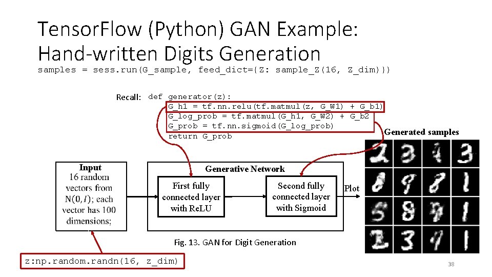
Tensor. Flow (Python) GAN Example: Hand-written Digits Generation samples = sess. run(G_sample, feed_dict={Z: sample_Z(16, Z_dim)}) Recall: def generator(z): G_h 1 = tf. nn. relu(tf. matmul(z, G_W 1) + G_b 1) G_log_prob = tf. matmul(G_h 1, G_W 2) + G_b 2 G_prob = tf. nn. sigmoid(G_log_prob) Generated samples return G_prob Input Generative Network First fully connected layer with Re. LU Second fully connected layer with Sigmoid Plot Fig. 13. GAN for Digit Generation z: np. random. randn(16, z_dim) 38

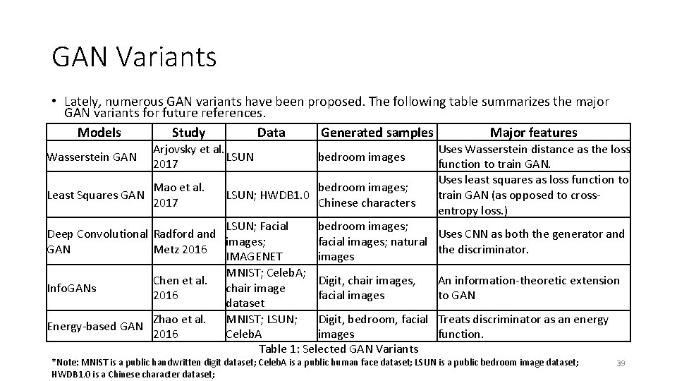
GAN Variants • Lately, numerous GAN variants have been proposed. The following table summarizes the major GAN variants for future references. Models Study Data Generated samples Major features Wasserstein GAN Arjovsky et al. LSUN 2017 bedroom images Least Squares GAN Mao et al. 2017 bedroom images; Chinese characters LSUN; HWDB 1. 0 LSUN; Facial bedroom images; Deep Convolutional Radford and images; facial images; natural GAN Metz 2016 IMAGENET images MNIST; Celeb. A; Chen et al. Digit, chair images, Info. GANs chair image 2016 facial images dataset Zhao et al. MNIST; LSUN; Digit, bedroom, facial Energy-based GAN 2016 Celeb. A images Table 1: Selected GAN Variants Uses Wasserstein distance as the loss function to train GAN. Uses least squares as loss function to train GAN (as opposed to crossentropy loss. ) Uses CNN as both the generator and the discriminator. An information-theoretic extension to GAN Treats discriminator as an energy function. *Note: MNIST is a public handwritten digit dataset; Celeb. A is a public human face dataset; LSUN is a public bedroom image dataset; HWDB 1. 0 is a Chinese character dataset; 39

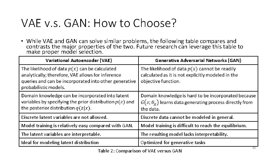
VAE v. s. GAN: How to Choose? • While VAE and GAN can solve similar problems, the following table compares and contrasts the major properties of the two. Future research can leverage this table to make proper model selection. Variational Autoencoder (VAE) Generative Adversarial Networks (GAN) Discrete latent variables are not allowed. Discrete data cannot be modeled in general. Model training is relatively easy compared with GAN. Model training is difficult to reach the equilibrium. The latent variables are interpretable. The resulting model lacks interpretability. Ideal for modeling latent distribution Optimized for generative tasks Table 2: Comparison of VAE versus GAN 40

Outline • Introduction • Traditional Generative Models • Deep Generative Models • Example Applications • Deep Belief Networks • Variational Autoencoder • Technical novelties • Implementation • Generative Adversarial Networks • Technical novelties • Implementation • Research Example: Motion Sensor-Based Fall Detection and Prediction • Conclusions • Appendix 41

Research Example Motion Sensor-Based Fall Detection and Prediction: A Hidden Markov Model and Generative Adversarial Network Approach Yidong Chai, Shuo Yu, Sagar Samtani, Hongyan Liu, Hsinchun Chen Artificial Intelligence Lab, The University of Arizona 42

Introduction • Population aging is a growing societal concern. • In 2015, 8. 5% of people worldwide (617 million) were aged 65 and over (NIH, 2015). • Falls are common among the elderly. • In the US, 28. 7% of senior citizens aged 65 and older fell in 2014. • Falls are threats to senior citizens. • Leading cause of injury/death among older Americans (CDC, 2016) • Fall risk assessment (detection and prediction) can alleviate threat of falls (Tong et al. 2013). • Prompt assistance can reduce the risk of hospitalization by 26% and death by over 80% (Scheffer et al. , 2008). • Wearable motion sensor-based systems for fall risk assessment • Components: data collection; data transmission; data analysis 43

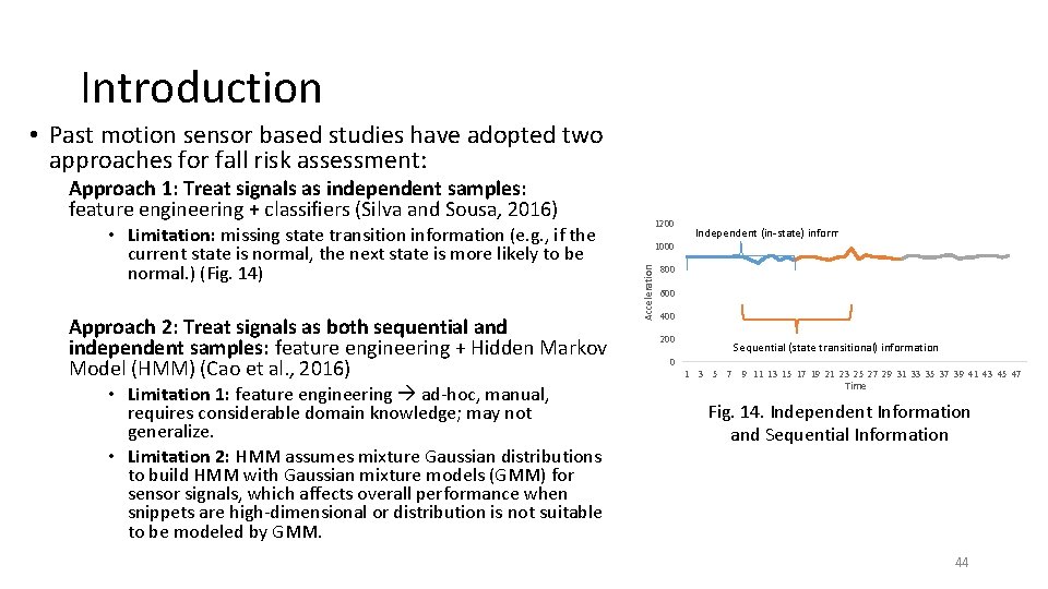
Introduction • Past motion sensor based studies have adopted two approaches for fall risk assessment: • Limitation: missing state transition information (e. g. , if the current state is normal, the next state is more likely to be normal. ) (Fig. 14) Approach 2: Treat signals as both sequential and independent samples: feature engineering + Hidden Markov Model (HMM) (Cao et al. , 2016) • Limitation 1: feature engineering ad-hoc, manual, requires considerable domain knowledge; may not generalize. • Limitation 2: HMM assumes mixture Gaussian distributions to build HMM with Gaussian mixture models (GMM) for sensor signals, which affects overall performance when snippets are high-dimensional or distribution is not suitable to be modeled by GMM. 1200 Independent (in-state) information 1000 Acceleration Approach 1: Treat signals as independent samples: feature engineering + classifiers (Silva and Sousa, 2016) 800 600 400 200 Sequential (state transitional) information 0 1 3 5 7 9 11 13 15 17 19 21 23 25 27 29 31 33 35 37 39 41 43 45 47 Time Fig. 14. Independent Information and Sequential Information 44

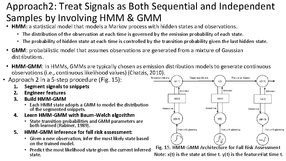
Approach 2: Treat Signals as Both Sequential and Independent Samples by Involving HMM & GMM • HMM: a statistical model that models a Markov process with hidden states and observations. • The distribution of the observation at each time is governed by the emission probability of each state. • The probability of hidden state at each time is controlled by the transition probability given the last hidden state. • GMM: probabilistic model that assumes observations are generated from a mixture of Gaussian distributions. • HMM-GMM: In HMMs, GMMs are typically chosen as emission distribution models to generate continuous observations (i. e. , continuous likelihood values) (Chatzis, 2010). • Approach 2 in a 5 -step procedure (Fig. 15): 1. 2. 3. Segment signals to snippets Engineer features Build HMM-GMM 4. Learn HMM-GMM with Baum-Welch algorithm 5. • Each HMM state adopts a GMM to model the distribution of the segmented snippets. • State transition probabilities and GMM parameters are both learned (Rabiner, 1989). HMM-GMM inference for fall risk assessment: • Given a new observation, infer the most likely state based on the trained model. • Predict the most likelihood state given the current inferred Fig. 15. HMM-GMM Architecture for Fall Risk Assessment 45 Note: x(t) is the state at time t. y(t) is the features at time t. state.

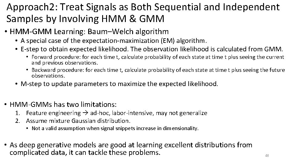
Approach 2: Treat Signals as Both Sequential and Independent Samples by Involving HMM & GMM • HMM-GMM Learning: Baum–Welch algorithm • A special case of the expectation-maximization (EM) algorithm. • E-step to obtain expected likelihood. The observation likelihood is calculated from GMM. • Forward procedure: for each time t, calculate probability of each state at time t plus seeing the current and previous observations. • Backward procedure: for each time t, calculate probability of each state at time t plus seeing the future observations. • M-step to update parameters to maximize the expected likelihood. • HMM-GMMs has two limitations: 1. Feature engineering ad-hoc, labor-intensive, may not generalize 2. Assume mixture Gaussian distribution. • Not a valid assumption when signal snippets increase in dimensionality. • As deep generative models are good at learning excellent distributions from complicated data, it can tackle these problems. 46

Deep Generative Models • Deep generative models obtain the joint probability of a sample and a label (i. e. , p(x, y)). This enables us to calculate the likelihood of sample given an label (i. e. , p(x|y)). • Analogous to the calculation of observation likelihood given the state, which is necessary for HMM learning and inference. • Therefore, we choose deep generative models in this research. • Common deep generative models include variational autoencoders (VAEs) and generative adversarial networks (GANs). • GANs have several advantages over VAEs: • GANs lead to the exact data distribution with infinite data and a large model, while VAEs may not lead to the exact data distribution even with infinite data and a large model. (Goodfellow, 2016) • GANs tend to generate better samples than the other deep learning models • Therefore, we focus on GANs in this research. 47

Literature Review – Likelihood Calculation Methods for Generative Adversarial Networks • While the GANs’ generative networks can address prevailing limitations of GMMs, they cannot directly replace GMMs in HMMs: • GANs lack an explicit probability distribution. Computing the exact likelihood is intractable. • Observation likelihood values are required by the conventional Baum-Welch algorithm for HMM learning (i. e. , the forward and backward procedures rely on observation likelihood values). • These limitations necessitate an approximation algorithm to obtain observation likelihoods. • Two prevailing methods can approximate likelihoods for GANs: Kernel Density Estimator (KDE) (Parzen, 1962) and Annealed Importance Sampling (AIS) (Neal, 2001) • Recent work notes AIS is preferred, as KDE is inaccurate with high-dimensional data (Wu et al. , 2017). • AIS is much more accurate than KDE (two orders of magnitude) (Wu et al. , 2017) 48

Research Gaps and Questions • We identified several domain and methodological gaps within extant literature. • Domain: Current approaches for fall risk assessment have several key drawbacks. • Independent samples: missing sequential (state transition) information • Sequential samples: feature engineering (ad-hoc, not generalizable) and GMM. • Methodological: • HMMs typically use GMMs to calculate observation likelihoods. • However, the mixture Gaussian assumption is not valid in some cases. • GANs learn distributions (Gaussian or otherwise) without feature engineering, but their likelihood is intractable (required by the Baum-Welch HMM training algorithm). • AIS can approximate observation likelihoods for GANs, but we are unaware of any approaches integrating this technique into an HMM. 49

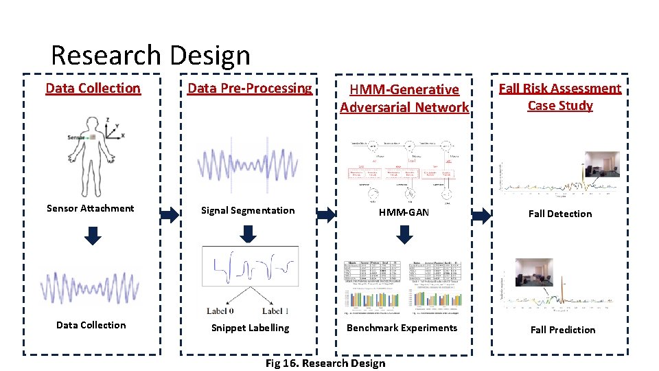
Research Gaps and Questions • These gaps motivate the following research questions: • Question 1: How can HMM’s GMM be replaced with a GAN such that both independent and sequential information can be captured from varying data distributions without manual feature engineering? • Question 2: How can AIS be used to generate likelihood values of GANs for subsequent integration into HMM training procedures? • Question 3: How can an integrated HMM-GAN model be used to improve performance fall risk assessment (detection and prediction) over the previous benchmark systems? • To answer these questions, we developed a novel fall risk assessment research framework with four major components (Fig. 16). 50

Research Design Data Collection Data Pre-Processing HMM-Generative Adversarial Network Fall Risk Assessment Case Study Sensor Attachment Signal Segmentation HMM-GAN Fall Detection Data Collection Snippet Labelling Benchmark Experiments Fall Prediction Fig 16. Research Design

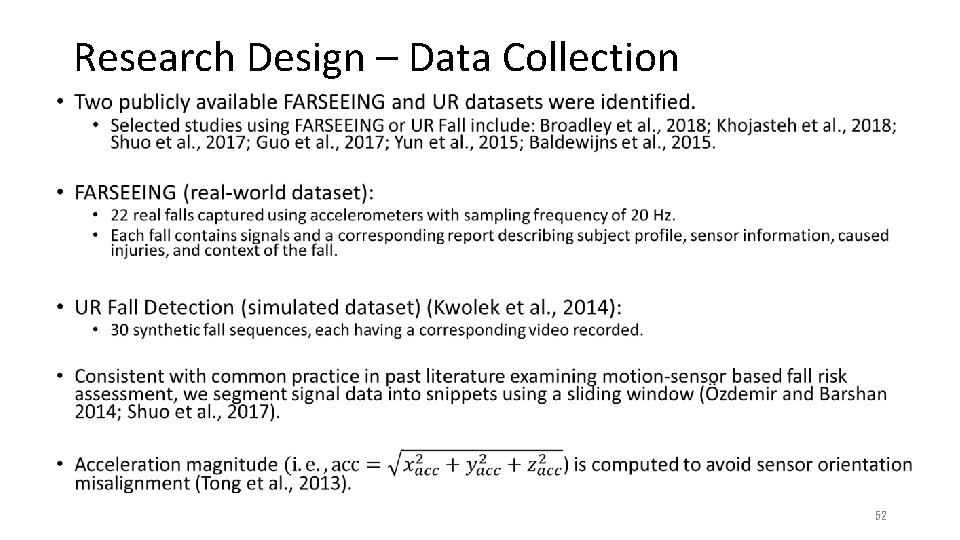
Research Design – Data Collection • 52

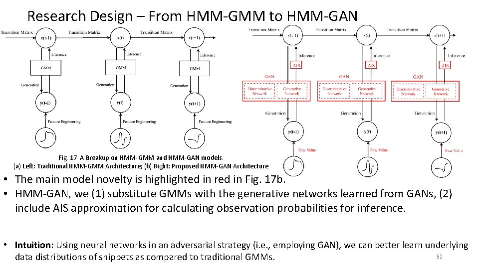
Research Design – From HMM-GMM to HMM-GAN Fig. 17 A Breakup on HMM-GMM and HMM-GAN models. (a) Left: Traditional HMM-GMM Architecture; (b) Right: Proposed HMM-GAN Architecture • The main model novelty is highlighted in red in Fig. 17 b. • HMM-GAN, we (1) substitute GMMs with the generative networks learned from GANs, (2) include AIS approximation for calculating observation probabilities for inference. • Intuition: Using neural networks in an adversarial strategy (i. e. , employing GAN), we can better learn underlying 53 data distributions of snippets as compared to traditional GMMs.

Research Design – Difficulty in HMM-GAN Training • The parameters of HMM-GAN (state transition probabilities and emission probabilities (i. e. , probability implied by GAN)) cannot be jointly obtained via the conventional Baum-Welch HMM learning algorithm. • No explicit probability distribution in GANs; therefore observation likelihoods are intractable (Goodfellow, 2016). • In the Baum-Welch algorithm, observation likelihood are required in the E-step (i. e. , the forward and backward procedure to calculate expectation likelihood). • Without an observation likelihood, E-step can not be implemented. As M-step is based on the output of E-step, both E-step and M-step cannot be implemented. • Therefore, HMM-GAN can not be learned in this way. 54

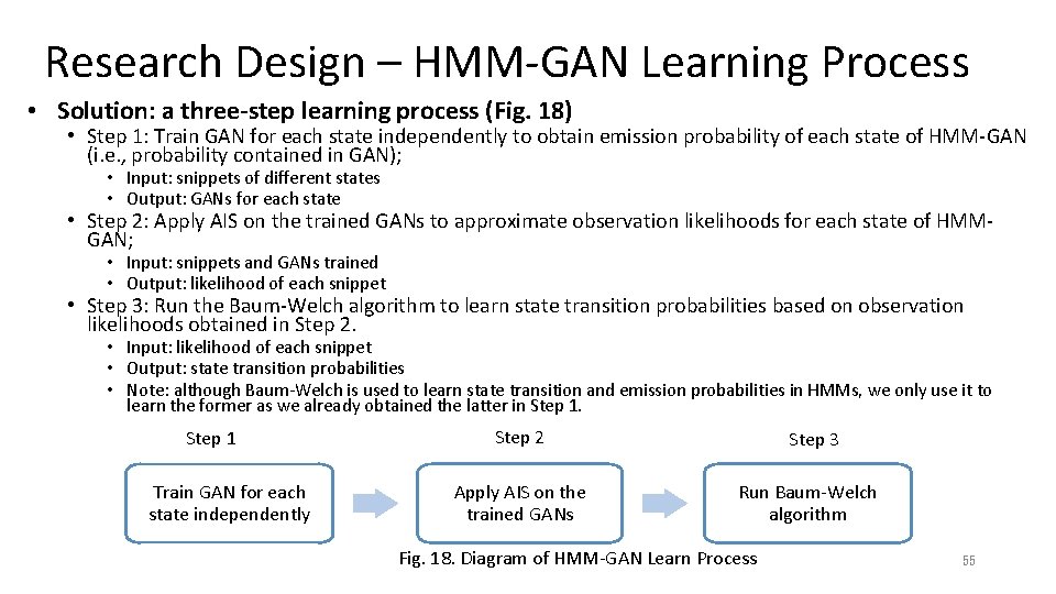
Research Design – HMM-GAN Learning Process • Solution: a three-step learning process (Fig. 18) • Step 1: Train GAN for each state independently to obtain emission probability of each state of HMM-GAN (i. e. , probability contained in GAN); • Input: snippets of different states • Output: GANs for each state • Step 2: Apply AIS on the trained GANs to approximate observation likelihoods for each state of HMMGAN; • Input: snippets and GANs trained • Output: likelihood of each snippet • Step 3: Run the Baum-Welch algorithm to learn state transition probabilities based on observation likelihoods obtained in Step 2. • Input: likelihood of each snippet • Output: state transition probabilities • Note: although Baum-Welch is used to learn state transition and emission probabilities in HMMs, we only use it to learn the former as we already obtained the latter in Step 1 Train GAN for each state independently Step 2 Step 3 Apply AIS on the trained GANs Run Baum-Welch algorithm Fig. 18. Diagram of HMM-GAN Learn Process 55

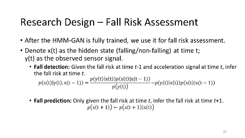
Research Design – Fall Risk Assessment • 56

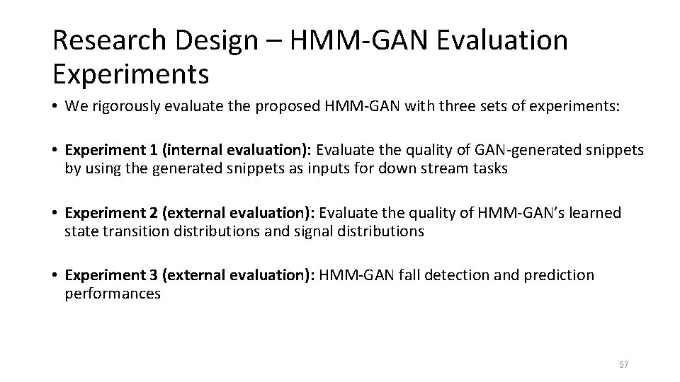
Research Design – HMM-GAN Evaluation Experiments • We rigorously evaluate the proposed HMM-GAN with three sets of experiments: • Experiment 1 (internal evaluation): Evaluate the quality of GAN-generated snippets by using the generated snippets as inputs for down stream tasks • Experiment 2 (external evaluation): Evaluate the quality of HMM-GAN’s learned state transition distributions and signal distributions • Experiment 3 (external evaluation): HMM-GAN fall detection and prediction performances 57

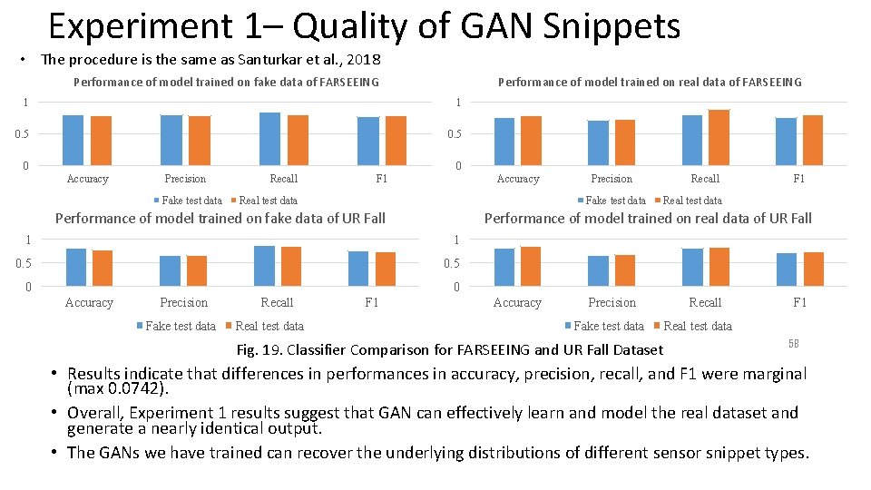
Experiment 1– Quality of GAN Snippets • The procedure is the same as Santurkar et al. , 2018 Performance of model trained on fake data of FARSEEING Performance of model trained on real data of FARSEEING 1 1 0. 5 0 0 Accuracy Precision Fake test data Recall F 1 Accuracy Real test data Fake test data Performance of model trained on fake data of UR Fall 1 0. 5 0 0 Precision Fake test data Recall Real test data F 1 Recall F 1 Real test data Performance of model trained on real data of UR Fall 1 Accuracy Precision Fake test data Fig. 19. Classifier Comparison for FARSEEING and UR Fall Dataset Recall F 1 Real test data 58 • Results indicate that differences in performances in accuracy, precision, recall, and F 1 were marginal (max 0. 0742). • Overall, Experiment 1 results suggest that GAN can effectively learn and model the real dataset and generate a nearly identical output. • The GANs we have trained can recover the underlying distributions of different sensor snippet types.

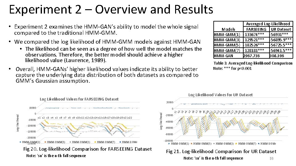
Experiment 2 – Overview and Results • Experiment 2 examines the HMM-GAN’s ability to model the whole signal compared to the traditional HMM-GMM. • We compared the log likelihood of HMM-GMM models against HMM-GAN • The likelihood can be seen as a degree of how well the model matches the observations. Therefore, the better model should achieve a higher likelihood value (Lawrence, 1989). • Overall, HMM-GANs’ higher likelihood values indicate its ability to better capture the underlying data distribution of both datasets as compared to GMM’s Gaussian assumption. 20000 50000 0 s 1 s 2 s 3 s 4 s 5 s 6 s 7 s 8 s 9 s 10 s 11 s 12 s 13 s 14 s 15 s 16 s 17 s 18 s 19 s 20 s 21 s 22 -100000 -150000 s 1 s 2 s 3 s 4 s 5 s 6 s 7 s 8 s 9 s 1 0 s 1 1 s 1 2 s 1 3 s 1 4 s 1 5 s 1 6 s 1 7 s 1 8 s 1 9 s 2 0 s 2 1 s 2 2 s 2 3 s 2 4 s 2 5 s 2 6 s 2 7 s 2 8 s 2 9 s 3 0 0 Log-likelihood Table 3. Averaged Log-likelihood Comparison Note: *** for p<0. 001 Log Likelihood Values for UR Dataset Log Likelihood Values for FARSEEING Dataset -50000 Models HMM-GMM(1) HMM-GMM(3) HMM-GMM(5) HMM-GMM(7) HMM-GAN Averaged Log-Likelihood FARSEEING UR Dataset -133674*** -56931*** -129521*** -56895. 9*** -182526*** -56725. 5*** -128181*** -56941. 5*** 2967. 736 308. 396 -20000 -40000 -60000 -80000 -200000 HMM-GMM(1) -250000 HMM-GMM(3) HMM-GMM(5) HMM-GMM(7) HMM-DGMs Fig 20. Log-likelihood Comparison for FARSEEING Dataset Note: ‘sn’ is the n-th fall sequence -100000 HMM-GMM(1) HMM-GMM(3) HMM-GMM(5) HMM-GMM(7) HMM-DGMs Fig 21. Log-likelihood Comparison for UR Dataset Note: ‘sn’ is the n-th fall sequence 59

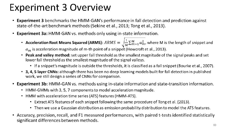
Experiment 3 Overview • 60

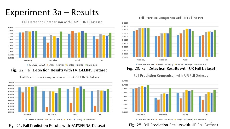
Experiment 3 a – Results Fall Detection Comparison with FARSEEING Dataset 1. 0000 0. 9000 0. 8000 0. 7000 0. 6000 0. 5000 0. 4000 0. 3000 0. 2000 0. 1000 0. 0000 Fall Detection Comparison with UR Fall Dataset 1. 0000 0. 9000 0. 8000 0. 7000 0. 6000 0. 5000 0. 4000 0. 3000 0. 2000 0. 1000 0. 0000 Accuracy Threshold method Precision ARMS Recall CNN(2) CNN(3) CNN(4) F 1 Threshold method HMM-GAN Fig. 22. Fall Detection Results with FARSEEING Dataset Precision ARMS CNN(2) Recall CNN(3) CNN(4) F 1 HMM-GAN Fig. 23. Fall Detection Results with UR Fall Dataset Fall Prediction Comparison with FARSEEING Dataset 1. 0000 0. 9000 0. 8000 0. 7000 0. 6000 0. 5000 0. 4000 0. 3000 0. 2000 0. 1000 0. 0000 Accuracy Threshold method Precision ARMS Recall CNN(2) CNN(3) CNN(4) F 1 HMM-GAN Fig. 24. Fall Prediction Results with FARSEEING Dataset Accuracy Threshold method Precision ARMS CNN(2) Recall CNN(3) CNN(4) F 1 HMM-GAN 61 Fig. 25. Fall Prediction Results with UR Fall Dataset

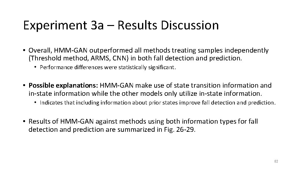
Experiment 3 a – Results Discussion • Overall, HMM-GAN outperformed all methods treating samples independently (Threshold method, ARMS, CNN) in both fall detection and prediction. • Performance differences were statistically significant. • Possible explanations: HMM-GAN make use of state transition information and in-state information while the other models only utilize in-state information. • Indicates that including information about prior states improve fall detection and prediction. • Results of HMM-GAN against methods using both information types for fall detection and prediction are summarized in Fig. 26 -29. 62

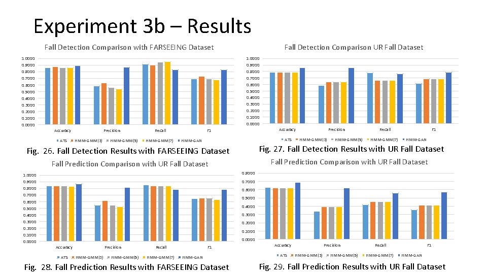
Experiment 3 b – Results Fall Detection Comparison with FARSEEING Dataset 1. 0000 0. 9000 0. 8000 0. 7000 0. 6000 0. 5000 0. 4000 0. 3000 0. 2000 0. 1000 0. 0000 Fall Detection Comparison UR Fall Dataset 1. 0000 0. 9000 0. 8000 0. 7000 0. 6000 0. 5000 0. 4000 0. 3000 0. 2000 0. 1000 0. 0000 Accuracy ATS Precision HMM-GMM(3) HMM-GMM(5) Recall HMM-GMM(7) F 1 Accuracy ATS HMM-GAN Precision HMM-GMM(3) HMM-GMM(5) Recall HMM-GMM(7) F 1 HMM-GAN Fig. 26. Fall Detection Results with FARSEEING Dataset Fig. 27. Fall Detection Results with UR Fall Dataset Fall Prediction Comparison with UR Fall Dataset 1. 0000 0. 9000 0. 8000 0. 7000 0. 6000 0. 5000 0. 4000 0. 3000 0. 2000 0. 1000 0. 0000 Accuracy ATS Precision HMM-GMM(3) HMM-GMM(5) Recall HMM-GMM(7) F 1 HMM-GAN Fig. 28. Fall Prediction Results with FARSEEING Dataset Accuracy ATS Precision HMM-GMM(3) HMM-GMM(5) Recall HMM-GMM(7) F 1 HMM-GAN Fig. 29. Fall Prediction Results with UR Fall Dataset

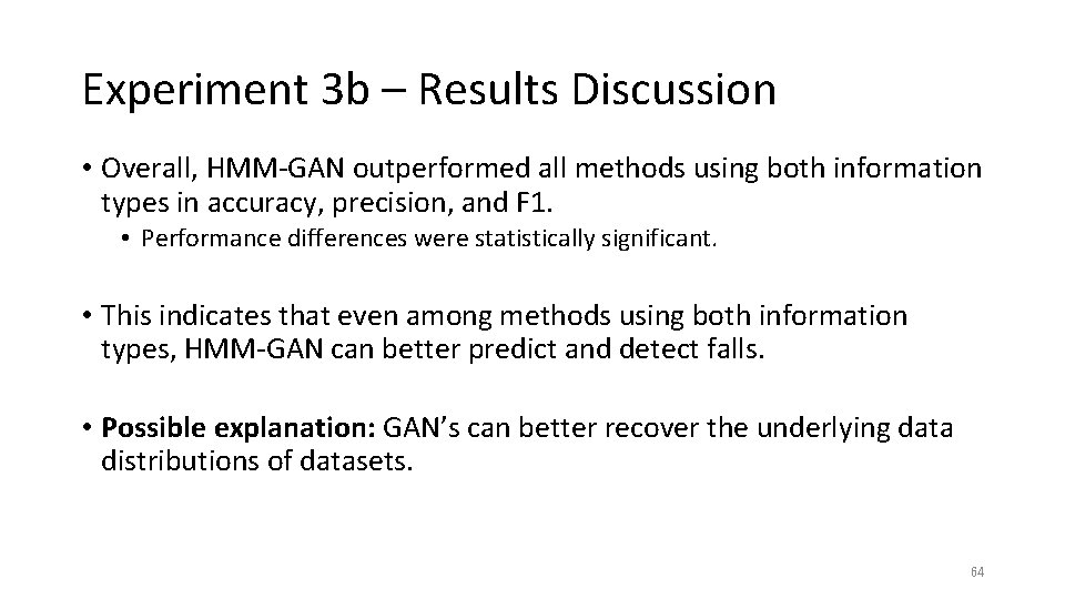
Experiment 3 b – Results Discussion • Overall, HMM-GAN outperformed all methods using both information types in accuracy, precision, and F 1. • Performance differences were statistically significant. • This indicates that even among methods using both information types, HMM-GAN can better predict and detect falls. • Possible explanation: GAN’s can better recover the underlying data distributions of datasets. 64

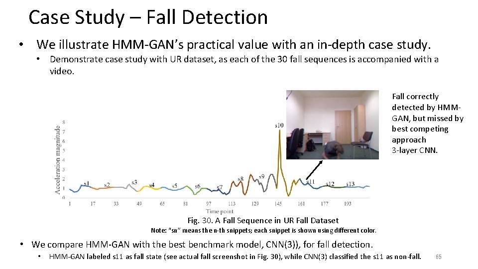
Case Study – Fall Detection • We illustrate HMM-GAN’s practical value with an in-depth case study. • Demonstrate case study with UR dataset, as each of the 30 fall sequences is accompanied with a video. Fall correctly detected by HMMGAN, but missed by best competing approach 3 -layer CNN. Fig. 30. A Fall Sequence in UR Fall Dataset Note: “sn” means the n-th snippets; each snippet is shown using different color. • We compare HMM-GAN with the best benchmark model, CNN(3)), for fall detection. • HMM-GAN labeled s 11 as fall state (see actual fall screenshot in Fig. 30), while CNN(3) classified the s 11 as non-fall. 65

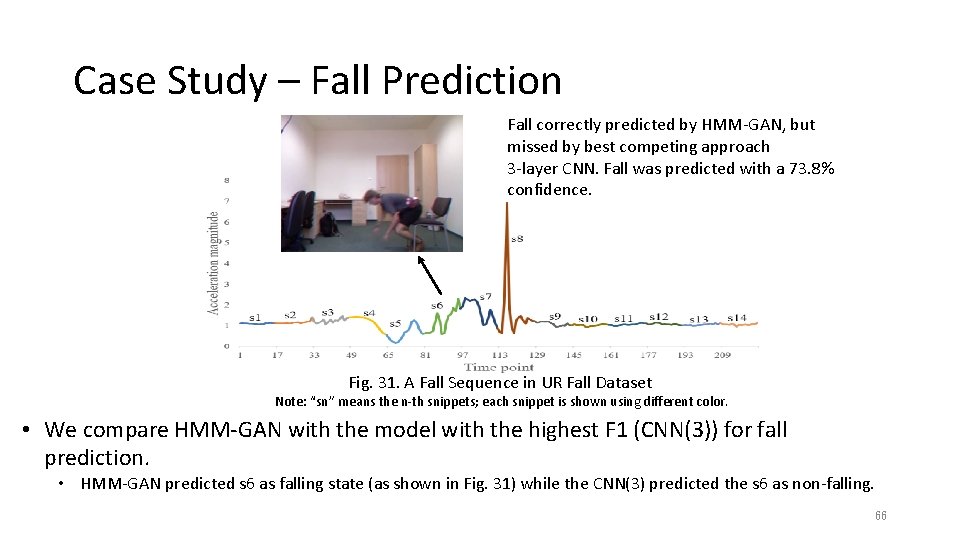
Case Study – Fall Prediction Fall correctly predicted by HMM-GAN, but missed by best competing approach 3 -layer CNN. Fall was predicted with a 73. 8% confidence. Fig. 31. A Fall Sequence in UR Fall Dataset Note: “sn” means the n-th snippets; each snippet is shown using different color. • We compare HMM-GAN with the model with the highest F 1 (CNN(3)) for fall prediction. • HMM-GAN predicted s 6 as falling state (as shown in Fig. 31) while the CNN(3) predicted the s 6 as non-falling. 66

Outline • Introduction • Traditional Generative Models • Deep Generative Models • Example Applications • Deep Belief Networks • Variational Autoencoder • Technical novelties • Implementation • Generative Adversarial Networks • Technical novelties • Implementation • Research Example: Motion Sensor-Based Fall Detection and Prediction • Conclusions • Appendix 67

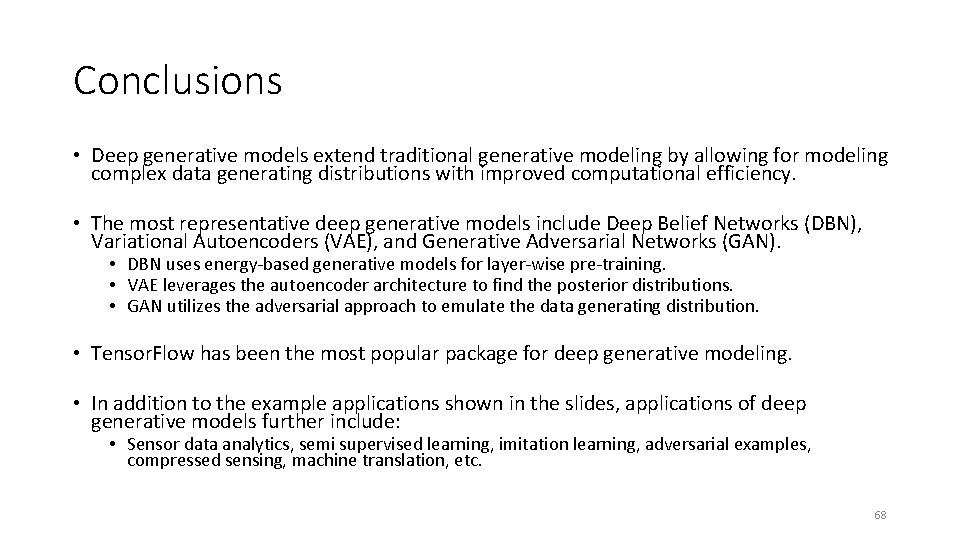
Conclusions • Deep generative models extend traditional generative modeling by allowing for modeling complex data generating distributions with improved computational efficiency. • The most representative deep generative models include Deep Belief Networks (DBN), Variational Autoencoders (VAE), and Generative Adversarial Networks (GAN). • DBN uses energy-based generative models for layer-wise pre-training. • VAE leverages the autoencoder architecture to find the posterior distributions. • GAN utilizes the adversarial approach to emulate the data generating distribution. • Tensor. Flow has been the most popular package for deep generative modeling. • In addition to the example applications shown in the slides, applications of deep generative models further include: • Sensor data analytics, semi supervised learning, imitation learning, adversarial examples, compressed sensing, machine translation, etc. 68

Outline • Introduction • Traditional Generative Models • Deep Generative Models • Example Applications • Deep Belief Networks • Variational Autoencoder • Technical novelties • Implementation • Generative Adversarial Networks • Technical novelties • Implementation • Research Example: Motion Sensor-Based Fall Detection and Prediction • Conclusions • Appendix 69

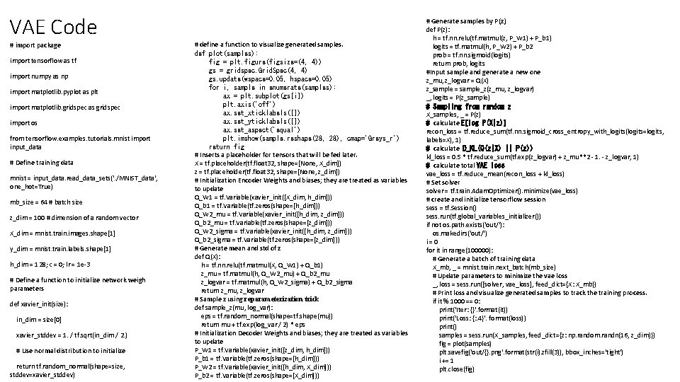
VAE Code # import package import tensorflow as tf import numpy as np import matplotlib. pyplot as plt import matplotlib. gridspec as gridspec import os from tensorflow. examples. tutorials. mnist import input_data # Define training data mnist = input_data. read_data_sets('. /MNIST_data', one_hot=True) mb_size = 64 # batch size z_dim = 100 # dimension of a random vector X_dim = mnist. train. images. shape[1] y_dim = mnist. train. labels. shape[1] h_dim = 128; c = 0; lr = 1 e-3 # Define a function to initialize network weigh parameters def xavier_init(size): in_dim = size[0] xavier_stddev = 1. / tf. sqrt(in_dim / 2. ) # Use normal distribution to initialize return tf. random_normal(shape=size, stddev=xavier_stddev) # define a function to visualize generated samples. def plot(samples): fig = plt. figure(figsize=(4, 4)) gs = gridspec. Grid. Spec(4, 4) gs. update(wspace=0. 05, hspace=0. 05) for i, sample in enumerate(samples): ax = plt. subplot(gs[i]) plt. axis('off') ax. set_xticklabels([]) ax. set_yticklabels([]) ax. set_aspect('equal') plt. imshow(sample. reshape(28, 28), cmap='Greys_r') return fig # Inserts a placeholder for tensors that will be fed later. X = tf. placeholder(tf. float 32, shape=[None, X_dim]) z = tf. placeholder(tf. float 32, shape=[None, z_dim]) # Initialization Encoder Weights and biases; they are treated as variables to update Q_W 1 = tf. Variable(xavier_init([X_dim, h_dim])) Q_b 1 = tf. Variable(tf. zeros(shape=[h_dim])) Q_W 2_mu = tf. Variable(xavier_init([h_dim, z_dim])) Q_b 2_mu = tf. Variable(tf. zeros(shape=[z_dim])) Q_W 2_sigma = tf. Variable(xavier_init([h_dim, z_dim])) Q_b 2_sigma = tf. Variable(tf. zeros(shape=[z_dim])) # Generate mean and std of z def Q(X): h = tf. nn. relu(tf. matmul(X, Q_W 1) + Q_b 1) z_mu = tf. matmul(h, Q_W 2_mu) + Q_b 2_mu z_logvar = tf. matmul(h, Q_W 2_sigma) + Q_b 2_sigma return z_mu, z_logvar # Sample z using reparameterization trick def sample_z(mu, log_var): eps = tf. random_normal(shape=tf. shape(mu)) return mu + tf. exp(log_var / 2) * eps # Initialization Decoder Weights and biases; they are treated as variables to update P_W 1 = tf. Variable(xavier_init([z_dim, h_dim])) P_b 1 = tf. Variable(tf. zeros(shape=[h_dim])) P_W 2 = tf. Variable(xavier_init([h_dim, X_dim])) P_b 2 = tf. Variable(tf. zeros(shape=[X_dim])) # Generate samples by P(z) def P(z): h = tf. nn. relu(tf. matmul(z, P_W 1) + P_b 1) logits = tf. matmul(h, P_W 2) + P_b 2 prob = tf. nn. sigmoid(logits) return prob, logits #Input sample and generate a new one z_mu, z_logvar = Q(X) z_sample = sample_z(z_mu, z_logvar) _, logits = P(z_sample) # Sampling from random z X_samples, _ = P(z) # calculate E[log P(X|z)] recon_loss = tf. reduce_sum(tf. nn. sigmoid_cross_entropy_with_logits(logits=logits, labels=X), 1) # calculate D_KL(Q(z|X) || P(z)) kl_loss = 0. 5 * tf. reduce_sum(tf. exp(z_logvar) + z_mu**2 - 1. - z_logvar, 1) # calculate total VAE loss vae_loss = tf. reduce_mean(recon_loss + kl_loss) # Set solver = tf. train. Adam. Optimizer(). minimize(vae_loss) # create and initialize tensorflow session sess = tf. Session() sess. run(tf. global_variables_initializer()) if not os. path. exists('out/'): os. makedirs('out/') i = 0 for it in range(100000): # Generate a batch of training data X_mb, _ = mnist. train. next_batch(mb_size) # Update parameters to minimize the vae loss _, loss = sess. run([solver, vae_loss], feed_dict={X: X_mb}) # Print loss and visualize generated samples to track the training process. if it % 1000 == 0: print('Iter: {}'. format(it)) print('Loss: {: . 4}'. format(loss)) print() samples = sess. run(X_samples, feed_dict={z: np. random. randn(16, z_dim)}) fig = plot(samples) plt. savefig('out/{}. png'. format(str(i). zfill(3)), bbox_inches='tight') i += 1 plt. close(fig)

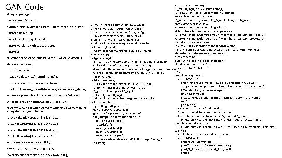
GAN Code # import package import tensorflow as tf from tensorflow. examples. tutorials. mnist import input_data import numpy as np import matplotlib. pyplot as plt import matplotlib. gridspec as gridspec import os # Define a function to initialize network weigh parameters def xavier_init(size): in_dim = size[0] xavier_stddev = 1. / tf. sqrt(in_dim / 2. ) # Use normal distribution to initialize return tf. random_normal(shape=size, stddev=xavier_stddev) # Inserts a placeholder for a tensor that will be fed later. X = tf. placeholder(tf. float 32, shape=[None, 784]) # weights and biases are treated as variables; add them to the computational graph to train D_W 1 = tf. Variable(xavier_init([784, 128])) D_b 1 = tf. Variable(tf. zeros(shape=[128])) D_W 2 = tf. Variable(xavier_init([128, 1])) D_b 2 = tf. Variable(tf. zeros(shape=[1])) # concatenate them for simplicity. theta_D = [D_W 1, D_W 2, D_b 1, D_b 2] Z = tf. placeholder(tf. float 32, shape=[None, 100]) G_sample = generator(Z) D_real, D_logit_real = discriminator(X) D_fake, D_logit_fake = discriminator(G_sample) # calculate discriminator loss D_loss = -tf. reduce_mean(tf. log(D_real) + tf. log(1. - D_fake)) # calculate generator loss G_W 1 = tf. Variable(xavier_init([100, 128])) G_loss = -tf. reduce_mean(tf. log(D_fake)) G_b 1 = tf. Variable(tf. zeros(shape=[128])) # Set solvers for discriminator and generator G_W 2 = tf. Variable(xavier_init([128, 784])) D_solver = tf. train. Adam. Optimizer(). minimize(D_loss, var_list=theta_D) G_b 2 = tf. Variable(tf. zeros(shape=[784])) G_solver = tf. train. Adam. Optimizer(). minimize(G_loss, var_list=theta_G) theta_G = [G_W 1, G_W 2, G_b 1, G_b 2] mb_size = 128 # batch size # define a function to sample a random vector Z_dim = 100 # dimension of the random vector def sample_Z(m, n): mnist = input_data. read_data_sets('. /MNIST_data', one_hot=True) return np. random. uniform(-1. , size=[m, n]) # create and initialize tensorflow session # generator(z) sess = tf. Session() def generator(z): sess. run(tf. global_variables_initializer()) # first fully connected operation with Re. LU transformation if not os. path. exists('out/'): G_h 1 = tf. nn. relu(tf. matmul(z, G_W 1) + G_b 1) # second fully connected operation with sigmoid transformation os. makedirs('out/') i = 0 G_prob = tf. nn. sigmoid (tf. matmul(G_h 1, G_W 2) + G_b 2) for it in range(100000): return G_prob if it % 1000 == 0: def discriminator(x): # Generate fake samples, i. e. , input Z and output G_sample D_h 1 = tf. nn. relu(tf. matmul(x, D_W 1) + D_b 1) samples = sess. run(G_sample, feed_dict={Z: sample_Z(16, Z_dim)}) D_logit = tf. matmul(D_h 1, D_W 2) + D_b 2 # Visualize the generated samples D_prob = tf. nn. sigmoid(D_logit) fig = plot(samples) return D_prob, D_logit plt. savefig('out/{}. png'. format(str(i). zfill(3)), bbox_inches='tight') # define a function to visualize generated samples. i += 1 def plot(samples): plt. close(fig) fig = plt. figure(figsize=(4, 4)) # Generate a batch of training data gs = gridspec. Grid. Spec(4, 4) X_mb, _ = mnist. train. next_batch(mb_size) gs. update(wspace=0. 05, hspace=0. 05) # Update parameters to minimize D_loss and G_loss for i, sample in enumerate(samples): _, D_loss_curr = sess. run([D_solver, D_loss], feed_dict={X: X_mb, Z: ax = plt. subplot(gs[i]) sample_Z(mb_size, Z_dim)}) plt. axis('off') _, G_loss_curr = sess. run([G_solver, G_loss], feed_dict={Z: sample_Z(mb_size, ax. set_xticklabels([]) Z_dim)}) ax. set_yticklabels([]) # Print loss to track the training process. ax. set_aspect('equal') if it % 1000 == 0: plt. imshow(sample. reshape(28, 28), cmap='Greys_r') print('Iter: {}'. format(it)) return fig print('D loss: {: . 4}'. format(D_loss_curr)) print('G_loss: {: . 4}'. format(G_loss_curr)) print()