Maxent Models and Discriminative Estimation Generative vs Discriminative

Maxent Models and Discriminative Estimation Generative vs. Discriminative models

Introduction So far we’ve looked at “generative models” Language models, Naive Bayes But there is now much use of conditional or discriminative probabilistic models in NLP, Speech, IR (and ML generally) Because: They give high accuracy performance They make it easy to incorporate lots of linguistically important features They allow automatic building of language independent, retargetable NLP modules

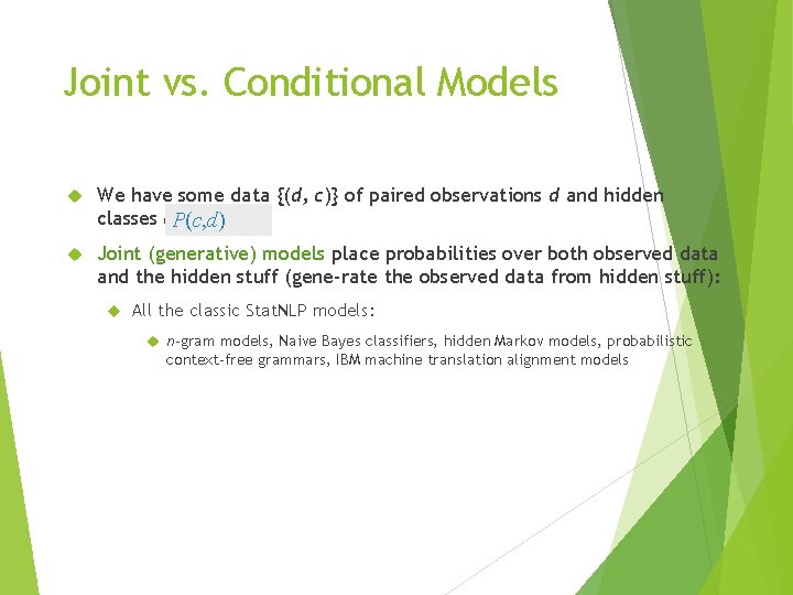
Joint vs. Conditional Models We have some data {(d, c)} of paired observations d and hidden classes c. P(c, d) Joint (generative) models place probabilities over both observed data and the hidden stuff (gene-rate the observed data from hidden stuff): All the classic Stat. NLP models: n-gram models, Naive Bayes classifiers, hidden Markov models, probabilistic context-free grammars, IBM machine translation alignment models

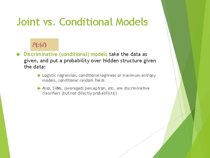
Joint vs. Conditional Models P(c|d) Discriminative (conditional) models take the data as given, and put a probability over hidden structure given the data: Logistic regression, conditional loglinear or maximum entropy models, conditional random fields Also, SVMs, (averaged) perceptron, etc. are discriminative classifiers (but not directly probabilistic)

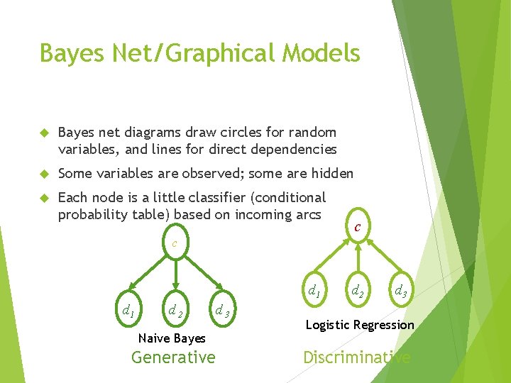
Bayes Net/Graphical Models Bayes net diagrams draw circles for random variables, and lines for direct dependencies Some variables are observed; some are hidden Each node is a little classifier (conditional probability table) based on incoming arcs c c d 1 d 2 Naive Bayes Generative d 3 d 2 d 3 Logistic Regression Discriminative

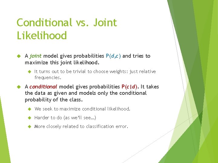
Conditional vs. Joint Likelihood A joint model gives probabilities P(d, c) and tries to maximize this joint likelihood. It turns out to be trivial to choose weights: just relative frequencies. A conditional model gives probabilities P(c|d). It takes the data as given and models only the conditional probability of the class. We seek to maximize conditional likelihood. Harder to do (as we’ll see…) More closely related to classification error.

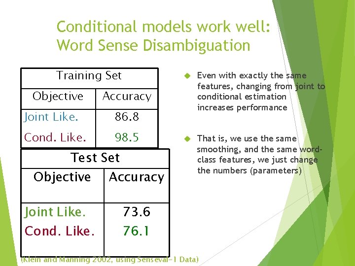
Conditional models work well: Word Sense Disambiguation Training Set Objective 86. 8 Cond. Like. 98. 5 Test Set Joint Like. Cond. Like. Even with exactly the same features, changing from joint to conditional estimation increases performance That is, we use the same smoothing, and the same wordclass features, we just change the numbers (parameters) Accuracy Joint Like. Objective Accuracy 73. 6 76. 1 (Klein and Manning 2002, using Senseval-1 Data)

Discriminative Model Features Making features from text for discriminative NLP models

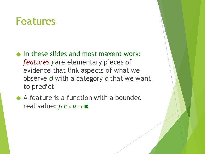
Features In these slides and most maxent work: features f are elementary pieces of evidence that link aspects of what we observe d with a category c that we want to predict A feature is a function with a bounded real value: f: C D → ℝ

Example features f 1(c, d) [c = LOCATION w-1 = “in” is. Capitalized(w)] f 2(c, d) [c = LOCATION has. Accented. Latin. Char(w)] f 3(c, d) [c = DRUG ends(w, “c”)] LOCATION in Arcadia LOCATION in Québec DRUG taking Zantac Models will assign to each feature a weight: A positive weight votes that this configuration is likely correct A negative weight votes that this configuration is likely incorrect PERSON saw Sue

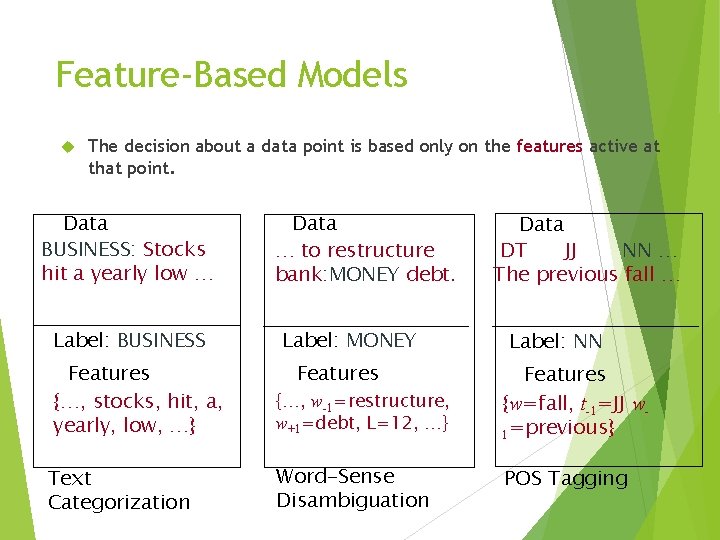
Feature-Based Models The decision about a data point is based only on the features active at that point. Data BUSINESS: Stocks hit a yearly low … Label: BUSINESS Features {…, stocks, hit, a, yearly, low, …} Text Categorization Data … to restructure bank: MONEY debt. Label: MONEY Features {…, w-1=restructure, w+1=debt, L=12, …} Word-Sense Disambiguation Data DT JJ NN … The previous fall … Label: NN Features {w=fall, t-1=JJ w 1=previous} POS Tagging

Feature-based (Log-Linear) Classifiers How to put features into a classifier 12

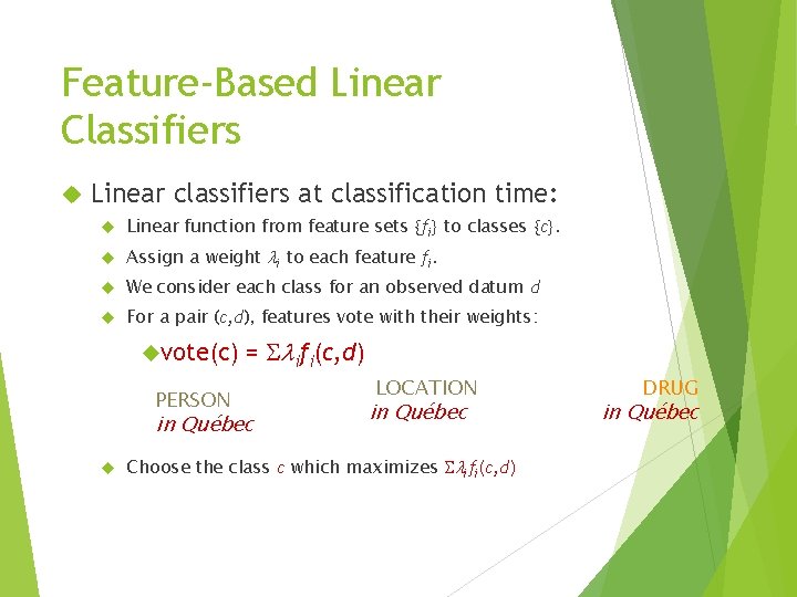
Feature-Based Linear Classifiers Linear classifiers at classification time: Linear function from feature sets {fi} to classes {c}. Assign a weight i to each feature fi. We consider each class for an observed datum d For a pair (c, d), features vote with their weights: vote(c) PERSON = ifi(c, d) in Québec LOCATION in Québec Choose the class c which maximizes ifi(c, d) DRUG in Québec

Feature-Based Linear Classifiers There are many ways to chose weights for features Perceptron: find a currently misclassified example, and nudge weights in the direction of its correct classification Margin-based methods (Support Vector Machines)

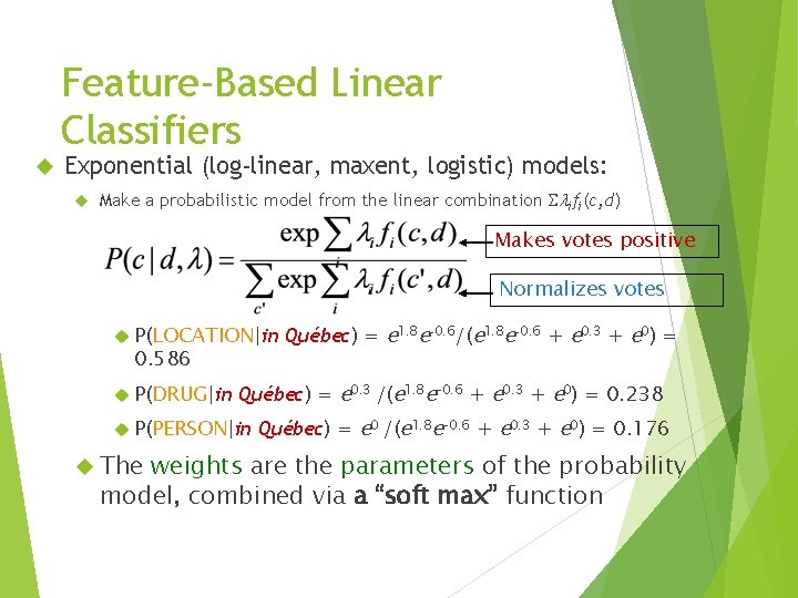
Feature-Based Linear Classifiers Exponential (log-linear, maxent, logistic) models: Make a probabilistic model from the linear combination ifi(c, d) Makes votes positive Normalizes votes P(LOCATION|in 0. 586 P(DRUG|in Québec) = e 0. 3 /(e 1. 8 e– 0. 6 + e 0. 3 + e 0) = 0. 238 P(PERSON|in The Québec) = e 1. 8 e– 0. 6/(e 1. 8 e– 0. 6 + e 0. 3 + e 0) = Québec) = e 0 /(e 1. 8 e– 0. 6 + e 0. 3 + e 0) = 0. 176 weights are the parameters of the probability model, combined via a “soft max” function

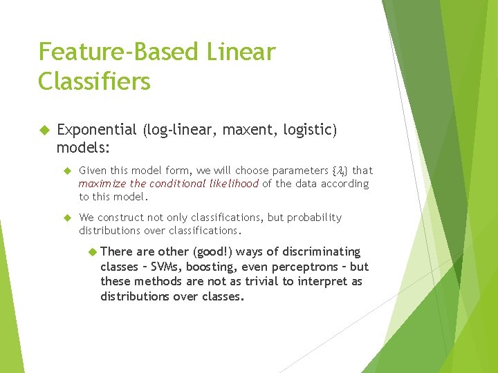
Feature-Based Linear Classifiers Exponential (log-linear, maxent, logistic) models: Given this model form, we will choose parameters { i} that maximize the conditional likelihood of the data according to this model. We construct not only classifications, but probability distributions over classifications. There are other (good!) ways of discriminating classes – SVMs, boosting, even perceptrons – but these methods are not as trivial to interpret as distributions over classes.

Aside: logistic regression Maxent models in NLP are essentially the same as multiclass logistic regression models in statistics (or machine learning) If you have seen these before you might think about: The parameterization is slightly different in a way that is advantageous for NLP- style models with tons of sparse features (but statistically inelegant) The key role of feature functions in NLP and in this presentation The features are more general, with f also being a function of the class – when might this be useful? 17

Building a Maxent Model The nuts and bolts

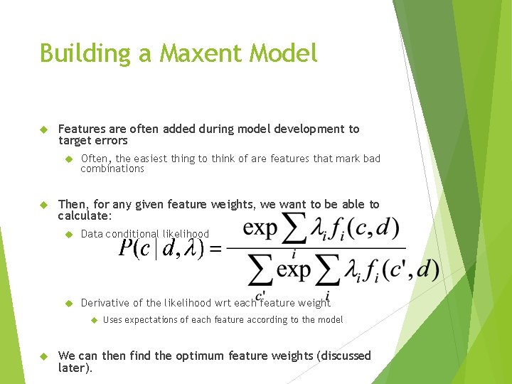
Building a Maxent Model Features are often added during model development to target errors Often, the easiest thing to think of are features that mark bad combinations Then, for any given feature weights, we want to be able to calculate: Data conditional likelihood Derivative of the likelihood wrt each feature weight Uses expectations of each feature according to the model We can then find the optimum feature weights (discussed later).

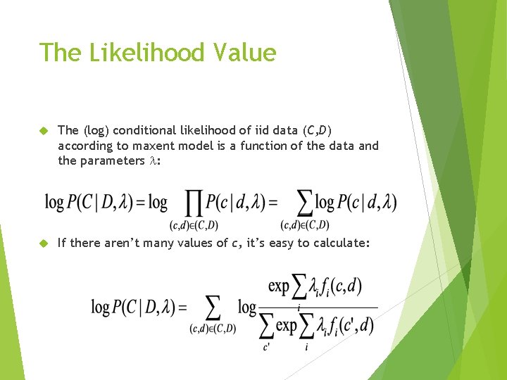
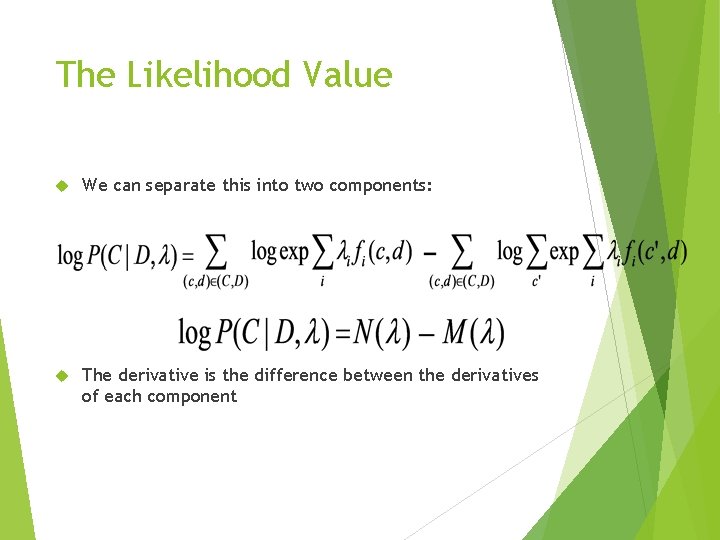
The Likelihood Value The (log) conditional likelihood of iid data (C, D) according to maxent model is a function of the data and the parameters : If there aren’t many values of c, it’s easy to calculate:

The Likelihood Value We can separate this into two components: The derivative is the difference between the derivatives of each component

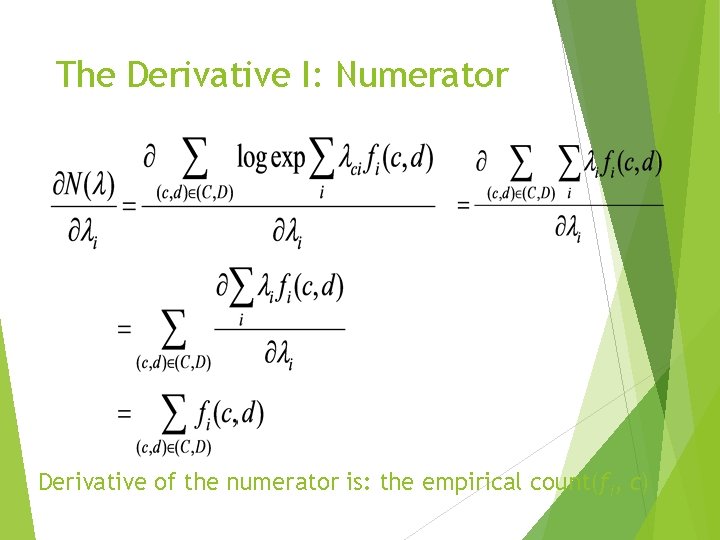
The Derivative I: Numerator Derivative of the numerator is: the empirical count(fi, c)

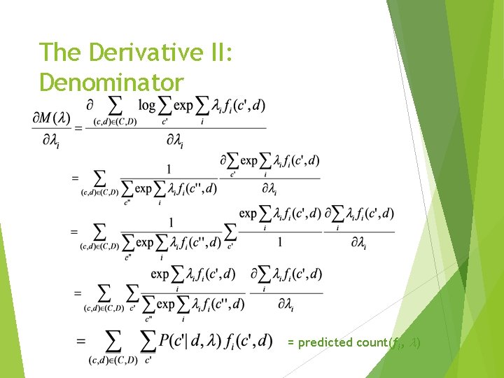
The Derivative II: Denominator = predicted count(fi, )

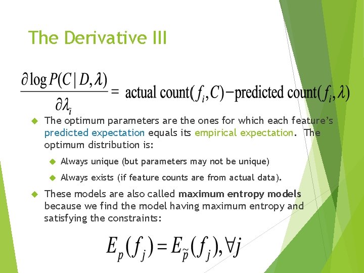
The Derivative III The optimum parameters are the ones for which each feature’s predicted expectation equals its empirical expectation. The optimum distribution is: Always unique (but parameters may not be unique) Always exists (if feature counts are from actual data). These models are also called maximum entropy models because we find the model having maximum entropy and satisfying the constraints:

Finding the optimal parameters Use your favorite numerical optimization package…. Commonly (and in our code), you minimize the negative of CLog. Lik 1. Gradient descent (GD); Stochastic gradient descent (SGD) 2. Iterative proportional fitting methods: Generalized Iterative Scaling (GIS) and Improved Iterative Scaling (IIS) 3. Conjugate gradient (CG), perhaps with preconditioning 4. Quasi-Newton methods – limited memory variable metric (LMVM) methods, in particular, L-BFGS

Smoothing/Priors/ Regularization for Maxent Models

Smoothing: Issues of Scale Lots of features: NLP maxent models can have well over a million features. Even storing a single array of parameter values can have a substantial memory cost. Lots of sparsity: Overfitting very easy – we need smoothing! Many features seen in training will never occur again at test time. Optimization problems: Feature weights can be infinite, and iterative solvers can take a long time to get to those infinities.

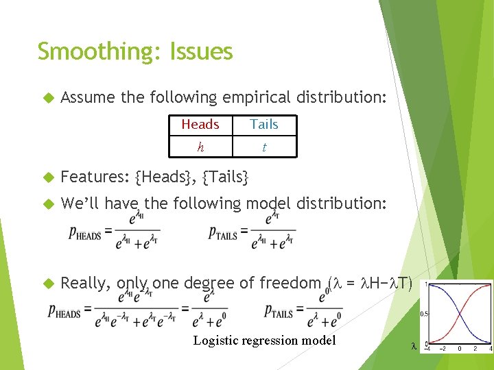
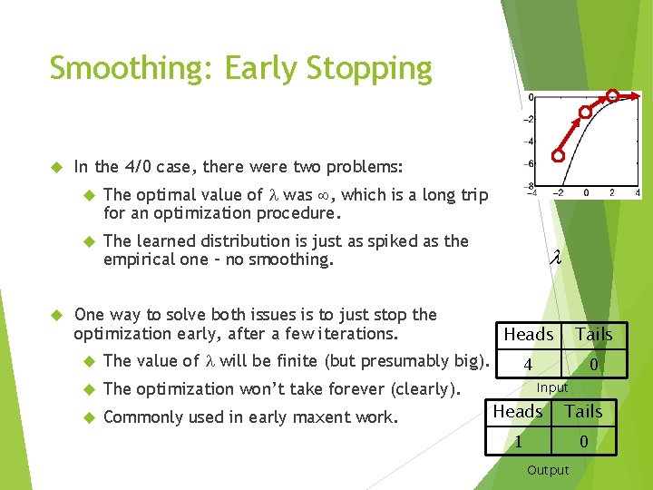
Smoothing: Issues Assume the following empirical distribution: Heads Tails h t Features: {Heads}, {Tails} We’ll have the following model distribution: Really, only one degree of freedom ( = H− T) Logistic regression model

Smoothing: Early Stopping In the 4/0 case, there were two problems: The optimal value of was , which is a long trip for an optimization procedure. The learned distribution is just as spiked as the empirical one – no smoothing. One way to solve both issues is to just stop the optimization early, after a few iterations. The value of will be finite (but presumably big). The optimization won’t take forever (clearly). Commonly used in early maxent work. Heads Tails 4 0 Input Heads Tails 1 0 Output

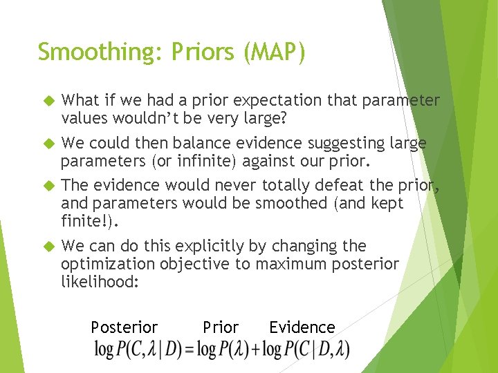
Smoothing: Priors (MAP) What if we had a prior expectation that parameter values wouldn’t be very large? We could then balance evidence suggesting large parameters (or infinite) against our prior. The evidence would never totally defeat the prior, and parameters would be smoothed (and kept finite!). We can do this explicitly by changing the optimization objective to maximum posterior likelihood: Posterior Prior Evidence

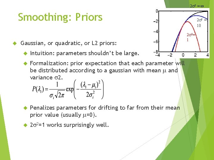
2 2 = Smoothing: Priors Gaussian, or quadratic, or L 2 priors: Intuition: parameters shouldn’t be large. Formalization: prior expectation that each parameter will be distributed according to a gaussian with mean and variance 2. Penalizes parameters for drifting to far from their mean prior value (usually =0). 2 2=1 works surprisingly well. 2 2 = 10 2 2= 1

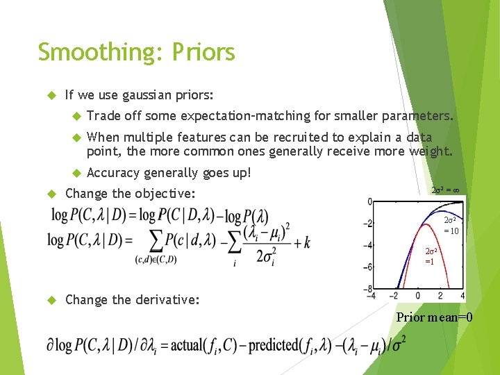
Smoothing: Priors If we use gaussian priors: Trade off some expectation-matching for smaller parameters. When multiple features can be recruited to explain a data point, the more common ones generally receive more weight. Accuracy generally goes up! Change the objective: 2 2 = 10 2 2 =1 Change the derivative: Prior mean=0

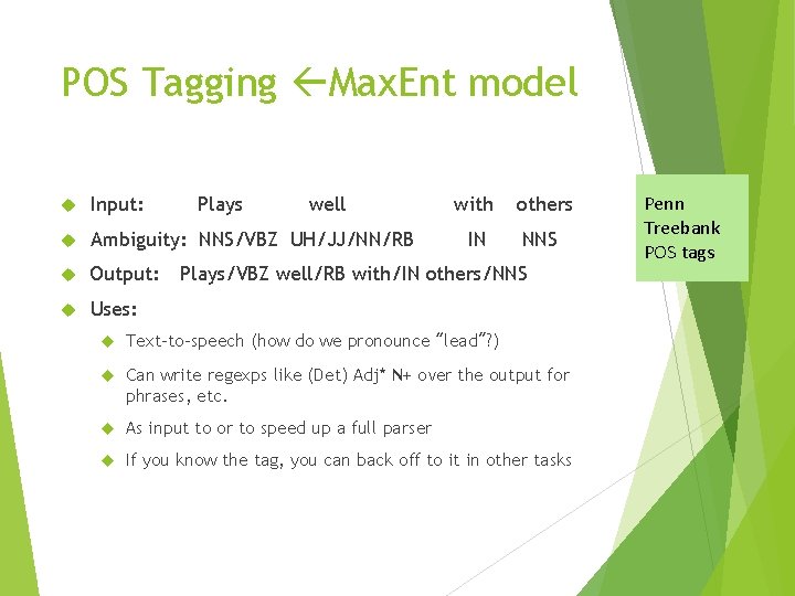
POS Tagging Max. Ent model Input: Plays well Ambiguity: NNS/VBZ UH/JJ/NN/RB Output: Uses: with others IN NNS Plays/VBZ well/RB with/IN others/NNS Text-to-speech (how do we pronounce “lead”? ) Can write regexps like (Det) Adj* N+ over the output for phrases, etc. As input to or to speed up a full parser If you know the tag, you can back off to it in other tasks Penn Treebank POS tags

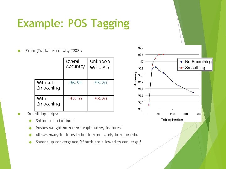
Example: POS Tagging From (Toutanova et al. , 2003): Overall Accuracy Unknown Word Acc Without Smoothing 96. 54 85. 20 With Smoothing 97. 10 88. 20 Smoothing helps: Softens distributions. Pushes weight onto more explanatory features. Allows many features to be dumped safely into the mix. Speeds up convergence (if both are allowed to converge)!

Smoothing: Regularization Talking of “priors” and “MAP estimation” is Bayesian language In frequentist statistics, people will instead talk about using “regularization”, and in particular, a gaussian prior is “L 2 regularization” The choice of names makes no difference to the math

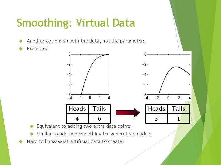
Smoothing: Virtual Data Another option: smooth the data, not the parameters. Example: Heads Tails 4 0 5 1 Equivalent to adding two extra data points. Similar to add-one smoothing for generative models. Hard to know what artificial data to create!

Smoothing: Count Cutoffs In NLP, features with low empirical counts are often dropped. Very weak and indirect smoothing method. Equivalent to locking their weight to be zero. Equivalent to assigning them gaussian priors with mean zero and variance zero. Dropping low counts does remove the features which were most in need of smoothing… … and speeds up the estimation by reducing model size … … but count cutoffs generally hurt accuracy in the presence of proper smoothing. We recommend: don’t use count cutoffs unless absolutely necessary for memory usage reasons.