DCM Theory 5 th March 2008 Andreina Mendez

DCM Theory 5 th March 2008 Andreina Mendez Stephanie Burnett

Recap • Last session: PPIs (psycho-physiological interactions) • Functional vs. effective connectivity – Functional connectivity: temporal correlation between spatially remote neurophysiological events Standard f. MRI analysis – Effective connectivity: the influence that the elements of a neuronal system exert over each other PPIs, SEM, DCM

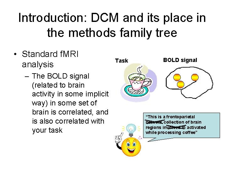
Introduction: DCM and its place in the methods family tree • Standard f. MRI analysis – The BOLD signal (related to brain activity in some implicit way) in some set of brain is correlated, and is also correlated with your task Task BOLD signal “This is a frontoparietal network collection of brain regions involved in activated while processing coffee”

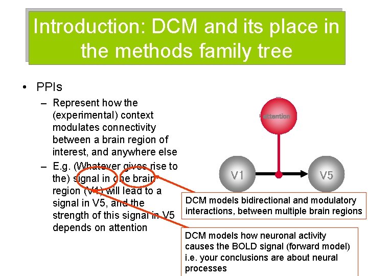
Introduction: DCM and its place in the methods family tree • PPIs – Represent how the (experimental) context attention modulates connectivity between a brain region of interest, and anywhere else – E. g. (Whatever gives rise to V 1 V 5 the) signal in one brain region (V 1) will lead to a DCM models bidirectional and modulatory signal in V 5, and the strength of this signal in V 5 interactions, between multiple brain regions depends on attention DCM models how neuronal activity causes the BOLD signal (forward model) i. e. your conclusions are about neural processes

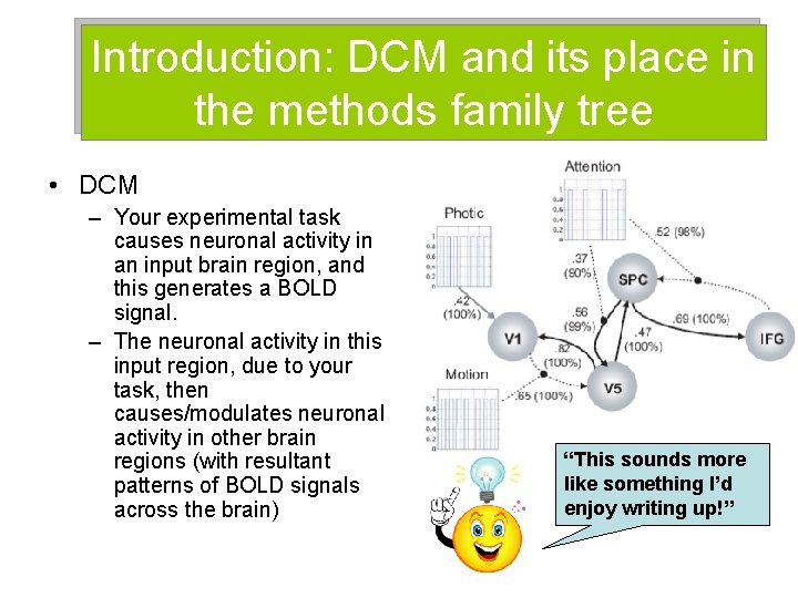
Introduction: DCM and its place in the methods family tree • DCM – Your experimental task causes neuronal activity in an input brain region, and this generates a BOLD signal. – The neuronal activity in this input region, due to your task, then causes/modulates neuronal activity in other brain regions (with resultant patterns of BOLD signals across the brain) “This sounds more like something I’d enjoy writing up!”

DCM basics • DCM models interactions between neuronal populations (f. MRI/MEG/EEG) • The aim is to estimate, and make inferences about, 1. The coupling among brain areas 2. How that coupling is influenced by changes in experimental context

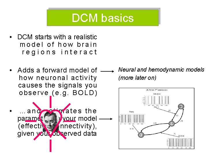
DCM basics • DCM starts with a realistic model of how brain regions interact • Adds a forward model of how neuronal activity causes the signals you observe (e. g. BOLD) • …and estimates the parameters in your model (effective connectivity), given your observed data Neural and hemodynamic models (more later on)

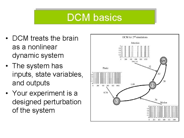
DCM basics • DCM treats the brain as a nonlinear dynamic system • The system has inputs, state variables, and outputs • Your experiment is a designed perturbation of the system

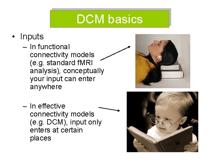
DCM basics • Inputs – In functional connectivity models (e. g. standard f. MRI analysis), conceptually your input can enter anywhere – In effective connectivity models (e. g. DCM), input only enters at certain places

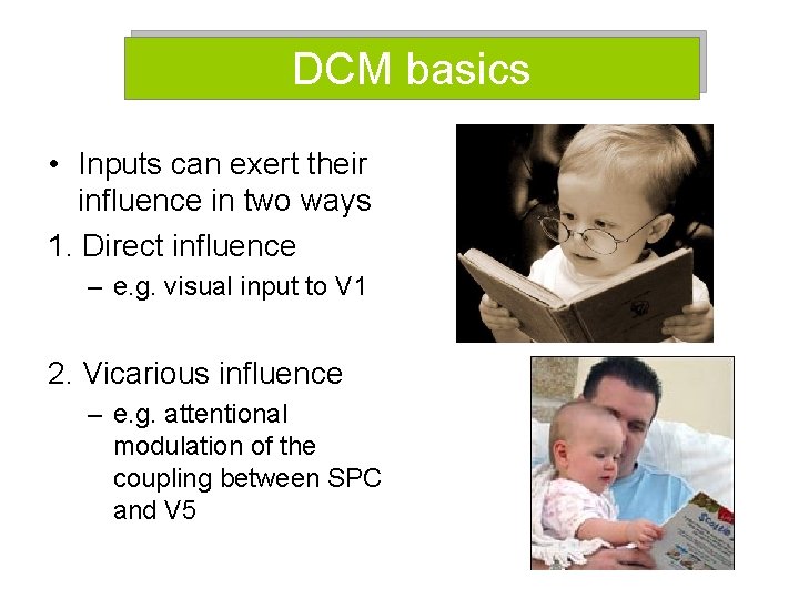
DCM basics • Inputs can exert their influence in two ways 1. Direct influence – e. g. visual input to V 1 2. Vicarious influence – e. g. attentional modulation of the coupling between SPC and V 5

DCM basics • State variables – neuronal activities, and other neuro/biophysical variables needed to form the outputs (later on) Neuronal priors Hemodynamic priors

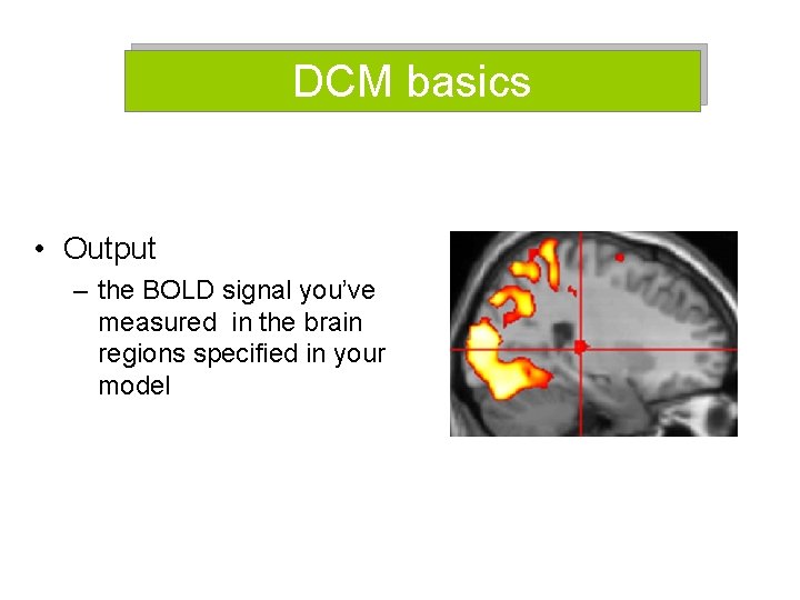
DCM basics • Output – the BOLD signal you’ve measured in the brain regions specified in your model

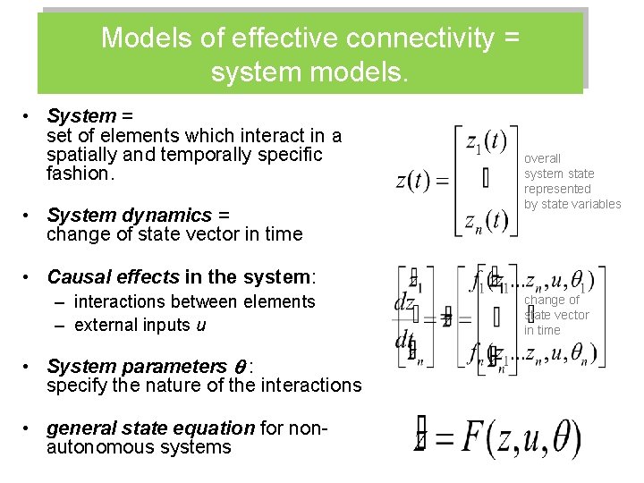
Models of effective connectivity = system models. • System = set of elements which interact in a spatially and temporally specific fashion. • System dynamics = change of state vector in time overall system state represented by state variables • Causal effects in the system: – interactions between elements – external inputs u • System parameters : specify the nature of the interactions • general state equation for nonautonomous systems change of state vector in time

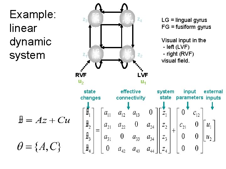
Example: linear dynamic system FG z 3 left LG z 1 left RVF u 2 state changes FG right z 4 LG right z 2 LG = lingual gyrus FG = fusiform gyrus Visual input in the - left (LVF) - right (RVF) visual field. LVF u 1 effective connectivity system input external state parameters inputs

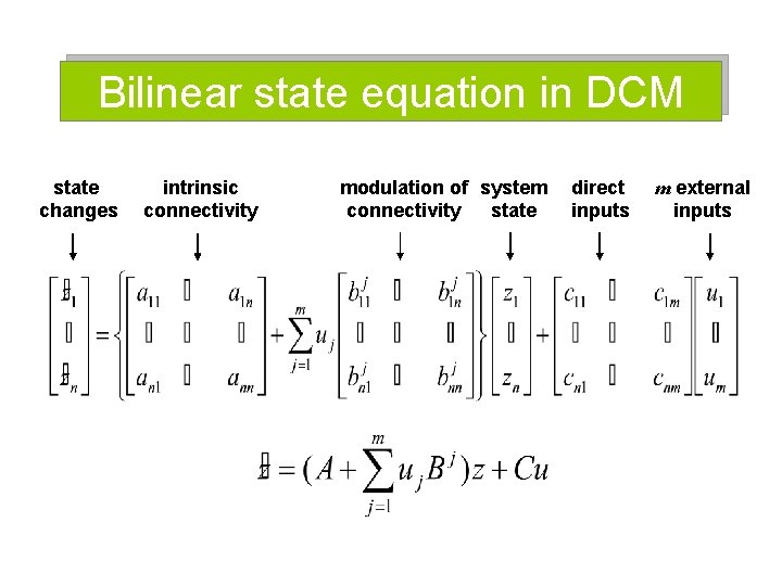
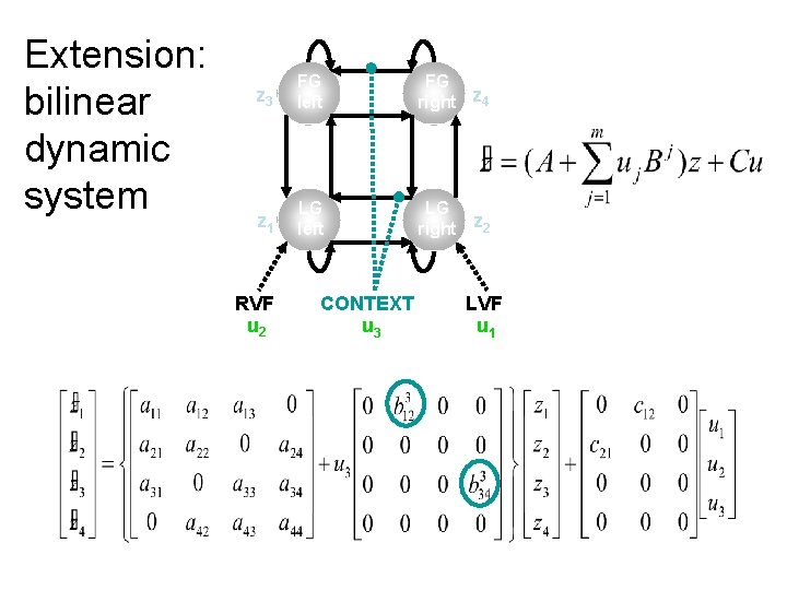
Bilinear state equation in DCM state changes intrinsic connectivity modulation of system connectivity state direct inputs m external inputs

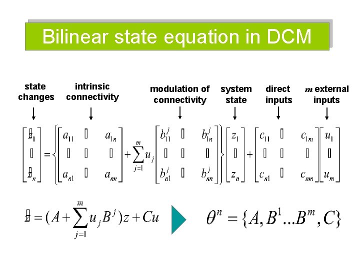
Bilinear state equation in DCM state changes intrinsic connectivity modulation of connectivity system state direct inputs m external inputs

Extension: bilinear dynamic system z 3 FG left FG right z 4 z 1 LG left LG right z 2 RVF u 2 CONTEXT u 3 LVF u 1

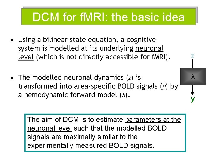
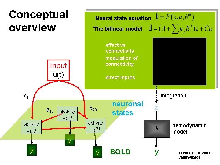
DCM for f. MRI: the basic idea • Using a bilinear state equation, a cognitive system is modelled at its underlying neuronal level (which is not directly accessible for f. MRI). • The modelled neuronal dynamics (z) is transformed into area-specific BOLD signals (y) by a hemodynamic forward model (λ). The aim of DCM is to estimate parameters at the neuronal level such that the modelled BOLD signals are maximally similar to the experimentally measured BOLD signals. z λ y

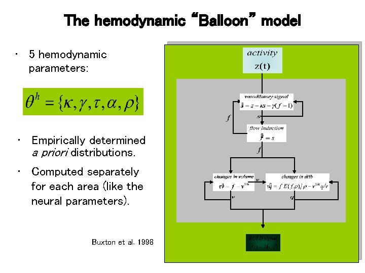
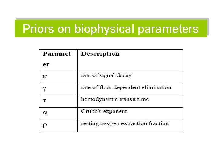
The hemodynamic “Balloon” model • 5 hemodynamic parameters: • Empirically determined a priori distributions. • Computed separately for each area (like the neural parameters). Buxton et al. 1998

Priors on biophysical parameters

Conceptual overview Neural state equation The bilinear model effective connectivity modulation of connectivity Input u(t) direct inputs c 1 integration a 12 activity z 2(t) activity z 1(t) b 23 neuronal states activity z 3(t) z λ hemodynamic model y y y BOLD y Friston et al. 2003, Neuro. Image

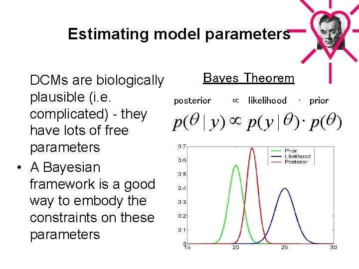
Estimating model parameters DCMs are biologically plausible (i. e. complicated) - they have lots of free parameters • A Bayesian framework is a good way to embody the constraints on these parameters Bayes Theorem posterior likelihood ∙ prior p(q | y ) p( y | q ) × p(q )

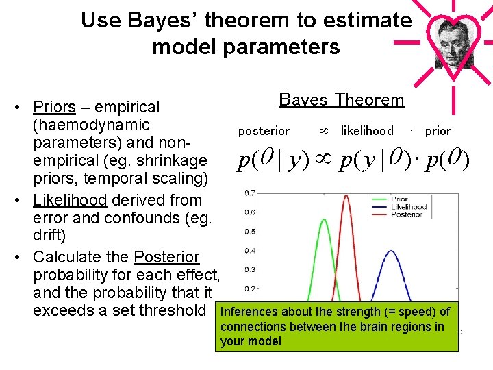
Use Bayes’ theorem to estimate model parameters Bayes Theorem • Priors – empirical (haemodynamic posterior likelihood ∙ prior parameters) and nonempirical (eg. shrinkage p(q | y ) p( y | q ) × p(q ) priors, temporal scaling) • Likelihood derived from error and confounds (eg. drift) • Calculate the Posterior probability for each effect, and the probability that it exceeds a set threshold Inferences about the strength (= speed) of connections between the brain regions in your model

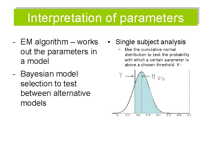
Interpretation of parameters - EM algorithm – works out the parameters in a model - Bayesian model selection to test between alternative models • Single subject analysis – Use the cumulative normal distribution to test the probability with which a certain parameter is above a chosen threshold γ: ηθ|y

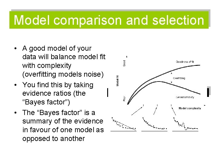
Model comparison and selection • A good model of your data will balance model fit with complexity (overfitting models noise) • You find this by taking evidence ratios (the “Bayes factor”) • The “Bayes factor” is a summary of the evidence in favour of one model as opposed to another

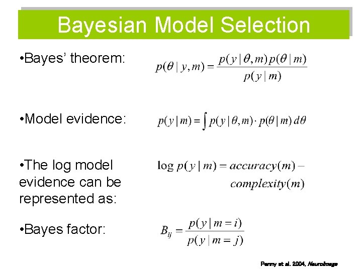
Bayesian Model Selection • Bayes’ theorem: • Model evidence: • The log model evidence can be represented as: • Bayes factor: Penny et al. 2004, Neuro. Image

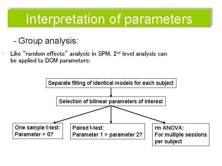
Interpretation of parameters - Group analysis: • Like “random effects” analysis in SPM, 2 nd level analysis can be applied to DCM parameters: Separate fitting of identical models for each subject Selection of bilinear parameters of interest One sample t-test: Parameter > 0? Paired t-test: Parameter 1 > parameter 2? rm ANOVA: For multiple sessions per subject

New stuff in DCM • 1. DCM now accounts for the slice timing problem

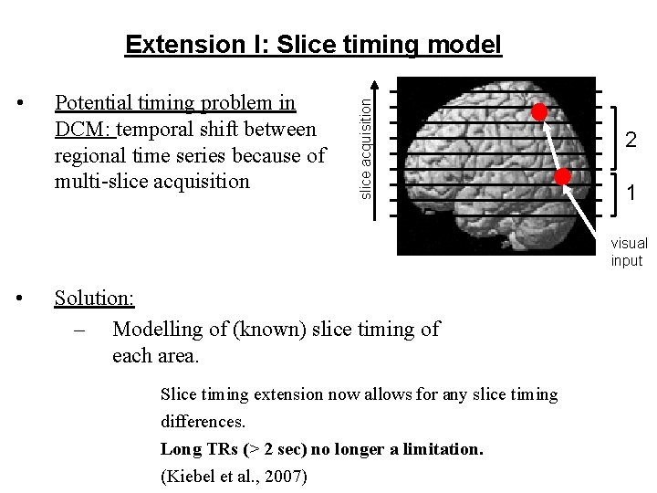
• Potential timing problem in DCM: temporal shift between regional time series because of multi-slice acquisition Extension I: Slice timing model 2 1 visual input • Solution: – Modelling of (known) slice timing of each area. Slice timing extension now allows for any slice timing differences. Long TRs (> 2 sec) no longer a limitation. (Kiebel et al. , 2007)

New stuff in DCM • 1. DCM now accounts for the slice timing problem (SPM 5) • 2. Biological plausibility: each brain area can have two states (SPM 8) (exc. /inh. )

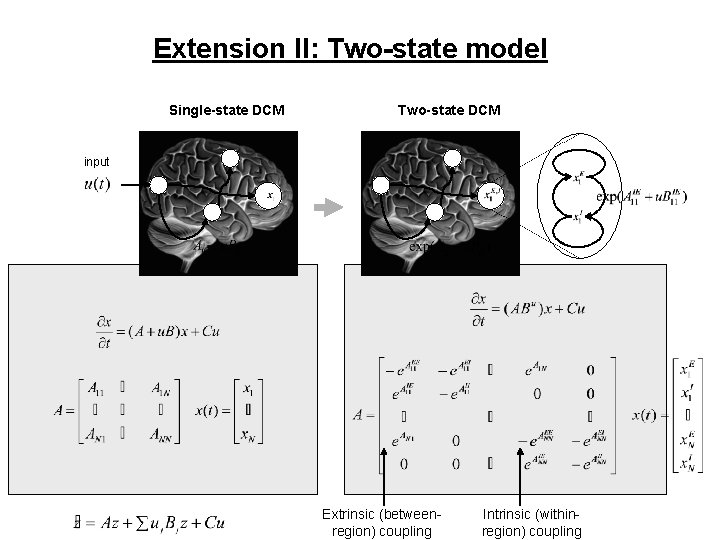
Extension II: Two-state model Single-state DCM Two-state DCM input Extrinsic (betweenregion) coupling Intrinsic (withinregion) coupling

New stuff in DCM • 1. DCM now accounts for the slice timing problem (SPM 5) • 2. Biological plausibility: each brain area can have two states (SPM 8) (exc. /inh. ) • 3. Biological plausibility: more complex balloon model (SPM 5) • 4. Non-linear version of DCM as well as bilinear (SPM 8)

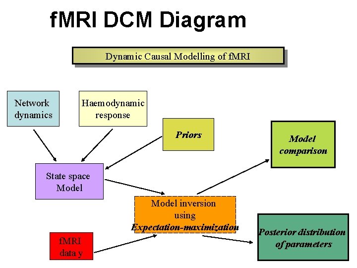
f. MRI DCM Diagram Dynamic Causal Modelling of f. MRI Network dynamics Haemodynamic response Priors Model comparison State space Model inversion using Expectation-maximization f. MRI data y Posterior distribution of parameters

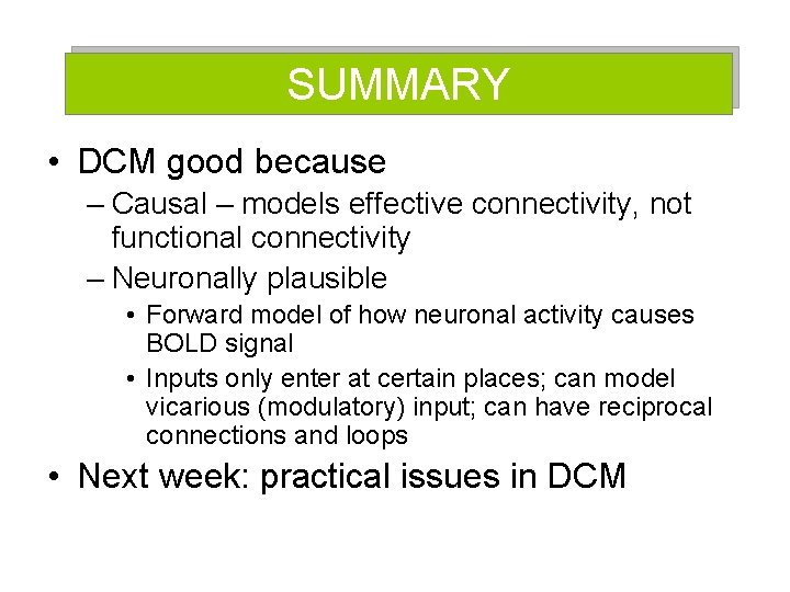
SUMMARY • DCM good because – Causal – models effective connectivity, not functional connectivity – Neuronally plausible • Forward model of how neuronal activity causes BOLD signal • Inputs only enter at certain places; can model vicarious (modulatory) input; can have reciprocal connections and loops • Next week: practical issues in DCM

REFERENCES • Karl J. Friston. Dynamic Causal Modelling. Human brain function. Chapter 22. Second Edition. http: //www. fil. ion. ucl. ac. uk/spm/doc/books/hbf 2/ • K. J Friston, L. Harrison and W. Penny. Dynamic Causal Modelling. Neuroimage 2003; 19: 12731302. • SPM Manual • Last year’s presentation

THANK YOU Special thanks to: - Andre Marreiros - Maria Joao