DCM for TimeFrequency 1 DCM for Induced Responses

DCM for Time-Frequency 1. DCM for Induced Responses 2. DCM for Phase Coupling Will Penny DCM Course, Paris, 2012

Dynamic Causal Models Neurophysiological Phenomenological Phase spiny stellate cells Pyramidal Cells Electromagnetic forward model included • DCM for ERP • DCM for SSR Frequency inhibitory interneurons Time Source locations not optimized • DCM for Induced Responses • DCM for Phase Coupling

1. DCM for Induced Responses Region 2 Frequency ? ? Time Frequency Region 1 Time Changes in power caused by external input and/or coupling with other regions Model comparisons: Which regions are connected? E. g. Forward/backward connections (Cross-)frequency coupling: Does slow activity in one region affect fast activity in another ?

Connection to Neural Mass Models First and Second order Volterra kernels From Neural Mass model. Strong (saturating) input leads to cross-frequency coupling

cf. Neural state equations in DCM for f. MRI Single region u 1 c a 11 z 1 u 2 z 1 z 2

cf. DCM for f. MRI Multiple regions u 1 c a 11 z 1 u 2 a 21 z 2 a 22 u 1 z 2

cf. DCM for f. MRI Modulatory inputs u 1 u 2 c u 1 a 11 z 1 b 21 a 21 z 2 a 22 u 2 z 1 z 2

cf. DCM for f. MRI Reciprocal connections u 1 u 2 c u 1 a 11 z 1 b 21 a 12 a 21 z 2 a 22 u 2 z 1 z 2

Frequency DCM for induced responses dg(t)/dt=A∙g(t)+C∙u(t) Time Where g(t) is a K x 1 vector of spectral responses A is a K x K matrix of frequency coupling parameters Also allow A to be changed by experimental condition

Frequency Use of Frequency Modes G=USV’ Time Where G is a K x T spectrogram U is K x K’ matrix with K frequency modes V is K x T and contains spectral mode responses over time Hence A is only K’ x K’, not K x K

Connection to Neurobiology From Neural Mass model. Strong (saturating) input leads to cross-frequency coupling

Connection to Neurobiology Strong (saturating) input leads to cross-frequency coupling

Connection to Neurobiology Weak input does not

Differential equation model for spectral energy Intrinsic (within-source) coupling Extrinsic (between-source) coupling Linear (within-frequency) coupling How frequency K in region j affects frequency 1 in region i Nonlinear (between-frequency) coupling

Modulatory connections Intrinsic (within-source) coupling Extrinsic (between-source) coupling

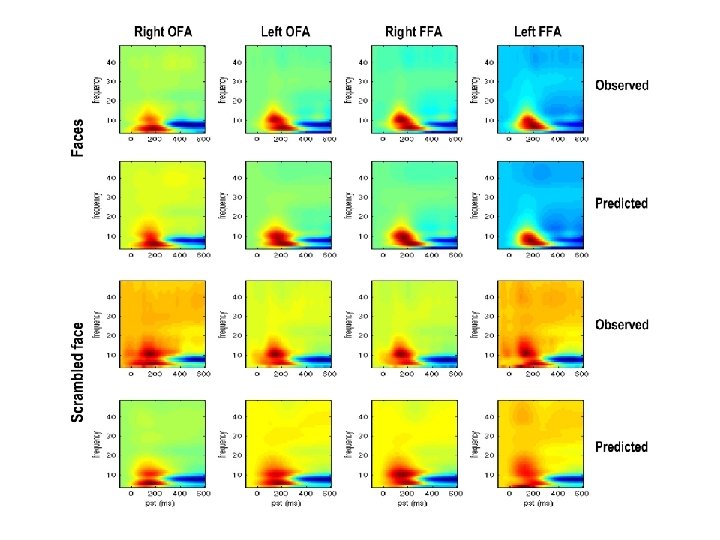
Example: MEG Data

The “core” system FFA OFA input

Face selective effects modulate within hemisphere forward and backward cxs linear nonlinear Backward Forward linear nonlinear F L BL F NB L F L NB F NB N F L BL F NB L nonlinear (and linear) linear F L BN F NB N FFA FFA OFA OFA Input

Model Inference Winning model: FNBN Both forward and backward connections are nonlinear FLBL FNBL FLBN *FNBN 0 1000 0 -10000 -20000 -16308 -16306 -11895 -2000 -30000 -40000 -5000 -6000 -50000 -7000 -60000 -70000 backward linear backward nonlinear -59890 -8000 forward linear forward nonlinear

Parameter Inference: gamma affects alpha Right backward - inhibitory suppressive effect of gamma-alpha coupling in backward connections SPM t df 72; FWHM 7. 8 x 6. 5 Hz 12 20 44 28 36 28 20 Frequency (Hz) 12 4 36 4 To 10 Hz Left forward - excitatory - activating effect of gamma-alpha coupling in the forward connections 44 From 30 Hz From 32 Hz (gamma) to 10 Hz (alpha) t = 4. 72; p = 0. 002

2. DCM for Phase Coupling For studying synchronization among brain regions Relate change of phase in one region to phase in others Region 2 Region 1 ? ? Phase Interaction Function Region 3

Region 2 Region 1 ? ? Synchronization achieved by phase coupling between regions Model comparisons: Which regions are connected? E. g. ‘master-slave’/mutual connections Parameter inference: (frequency-dependent) coupling values

Synchronization Gamma sync synaptic plasticity, forming ensembles Theta sync system-wide distributed control (phase coding) Pathological (epilepsy, Parkinsons) Phase Locking Indices, Phase Lag etc are useful characterising systems in their steady state Sync – Steve Strogatz

One Oscillator

Two Oscillators

Two Coupled Oscillators 0. 3 Here we assume the Phase Interaction Function (PIF) is a sinewave

Different initial phases 0. 3

Stronger coupling 0. 6

Bidirectional coupling 0. 3

DCM for Phase Coupling Allow connections to depend on experimental condition Phase interaction function is an arbitrary order Fourier series

Example: MEG data Fuentemilla et al, Current Biology, 2010

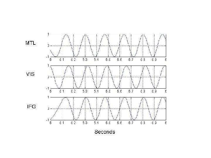
Delay activity (4 -8 Hz) Visual Cortex (VIS) Medial Temporal Lobe (MTL) Inferior Frontal Gyrus (IFG)

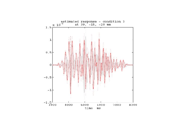
Questions • Duzel et al. find different patterns of theta-coupling in the delay period dependent on task. • Pick 3 regions based on [previous source reconstruction] 1. Right MTL [27, -18, -27] mm 2. Right VIS [10, -100, 0] mm 3. Right IFG [39, 28, -12] mm • Find out if structure of network dynamics is Master-Slave (MS) or (Partial/Total) Mutual Entrainment (ME) • Which connections are modulated by memory task ?

MTL Master. Slave 1 IFG VIS Master VIS 3 IFG Partial Mutual Entrainment VIS 5 IFG MTL 2 IFG Master IFG VIS 4 IFG MTL Total Mutual Entrainment MTL VIS MTL 6 IFG VIS MTL 7 IFG VIS

Analysis • Source reconstruct activity in areas of interest (with fewer sources than sensors and known location, then pinv will do; Baillet 01) • Bandpass data into frequency range of interest • Hilbert transform data to obtain instantaneous phase. Data that we model are unwrapped phase time series in multiple regions. • Use multiple trials per experimental condition • Model inversion

3 IFG VIS MTL Log. Ev Model

Connection Strengths 0. 77 IFG 2. 46 VIS 2. 89 MTL 0. 89

Recordings from rats doing spatial memory task: Jones and Wilson, PLo. S B, 2005

f. IFG-f. VIS Control f. MTL-f. VIS

f. IFG-f. VIS Memory f. MTL-f. VIS

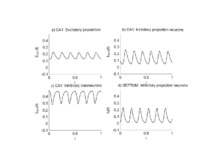
Connection to Neurobiology: Septo-Hippocampal theta rhythm Denham et al. 2000: Wilson-Cowan style model Hippocampus Septum

Four-dimensional state space

Hopf Bifurcation Hippocampus A B Septum A B

For a generic Hopf bifurcation (Erm & Kopell…) See Brown et al. 04, for PRCs corresponding to other bifurcations