CSC D 70 Compiler Optimization Prof Gennady Pekhimenko

CSC D 70: Compiler Optimization Prof. Gennady Pekhimenko University of Toronto Winter 2018 The content of this lecture is adapted from the lectures of Todd Mowry and Phillip Gibbons

CSC D 70: Compiler Optimization Introduction, Logistics Prof. Gennady Pekhimenko University of Toronto Winter 2018 The content of this lecture is adapted from the lectures of Todd Mowry and Phillip Gibbons

Summary • Syllabus – Course Introduction, Logistics, Grading • Information Sheet – Getting to know each other • Assignments • Learning LLVM • Compiler Basics 3

Syllabus: Who Are We? 4

Gennady (Gena) Pekhimenko Assistant Professor, Instructor pekhimenko@cs. toronto. edu http: //www. cs. toronto. edu/~pekhimenko/ Office: BA 5232 / IC 454 Ph. D from Carnegie Mellon Worked at Microsoft Research, NVIDIA, IBM Research interests: computer architecture, systems, machine learning, compilers, hardware acceleration, bioinformatics Computer Systems and Networking Group (CSNG) Eco. System Group

Bojian Zheng MSc. Student, TA bojian@cs. toronto. edu Office: BA 5214 D 02 BSc. from Uof. T ECE Research interests: computer architecture, GPUs, machine learning Computer Systems and Networking Group (CSNG) Eco. System Group

Course Information: Where to Get? • Course Website: http: //www. cs. toronto. edu/~pekhimenko/courses/cscd 70 w 18/ – Announcements, Syllabus, Course Info, Lecture Notes, Tutorial Notes, Assignments • Piazza: https: //piazza. com/utoronto. ca/winter 2018/cscd 70/home – Questions/Discussions, Syllabus, Announcements • Blackboard – Emails/announcements • Your email 7

Useful Textbook 8

CSC D 70: Compiler Optimization Compiler Introduction Prof. Gennady Pekhimenko University of Toronto Winter 2018 The content of this lecture is adapted from the lectures of Todd Mowry and Phillip Gibbons

Introduction to Compilers • What would you get out of this course? • Structure of a Compiler • Optimization Example 10

What Do Compilers Do? 1. Translate one language into another – e. g. , convert C++ into x 86 object code – difficult for “natural” languages, but feasible for computer languages 2. Improve (i. e. “optimize”) the code – e. g. , make the code run 3 times faster • or more energy efficient, more robust, etc. – driving force behind modern processor design 11

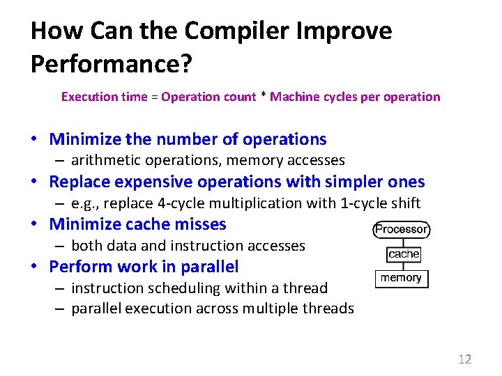
How Can the Compiler Improve Performance? Execution time = Operation count * Machine cycles per operation • Minimize the number of operations – arithmetic operations, memory accesses • Replace expensive operations with simpler ones – e. g. , replace 4 -cycle multiplication with 1 -cycle shift • Minimize cache misses – both data and instruction accesses • Perform work in parallel – instruction scheduling within a thread – parallel execution across multiple threads 12

What Would You Get Out of This Course? • Basic knowledge of existing compiler optimizations • Hands-on experience in constructing optimizations within a fully functional research compiler • Basic principles and theory for the development of new optimizations 13

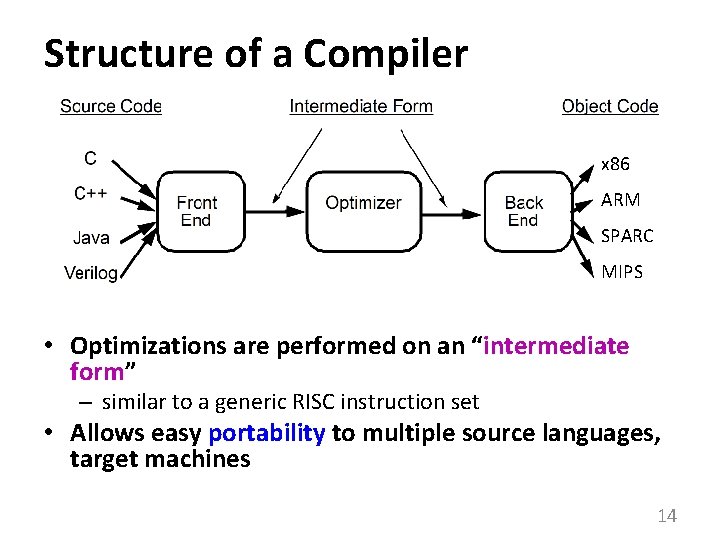
Structure of a Compiler x 86 ARM SPARC MIPS • Optimizations are performed on an “intermediate form” – similar to a generic RISC instruction set • Allows easy portability to multiple source languages, target machines 14

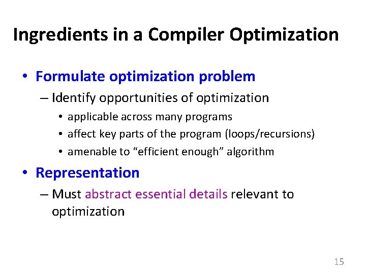
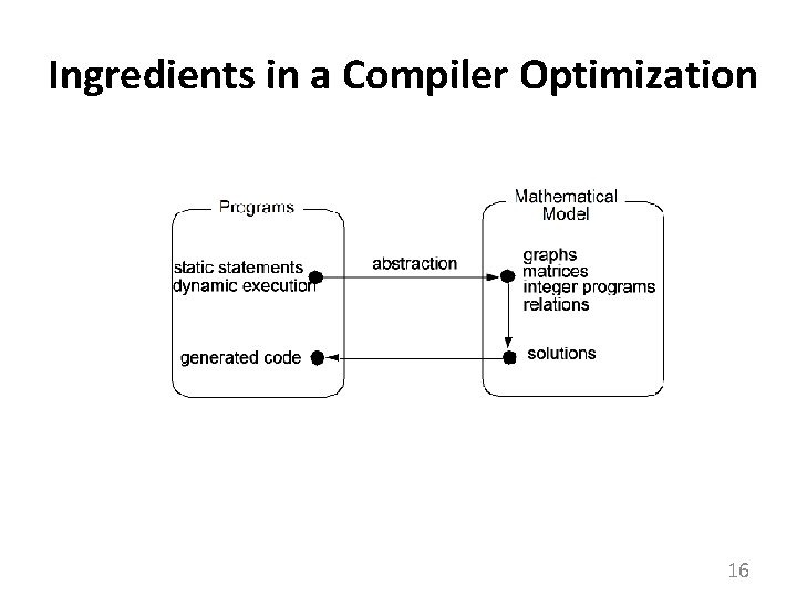
Ingredients in a Compiler Optimization • Formulate optimization problem – Identify opportunities of optimization • applicable across many programs • affect key parts of the program (loops/recursions) • amenable to “efficient enough” algorithm • Representation – Must abstract essential details relevant to optimization 15

Ingredients in a Compiler Optimization 16

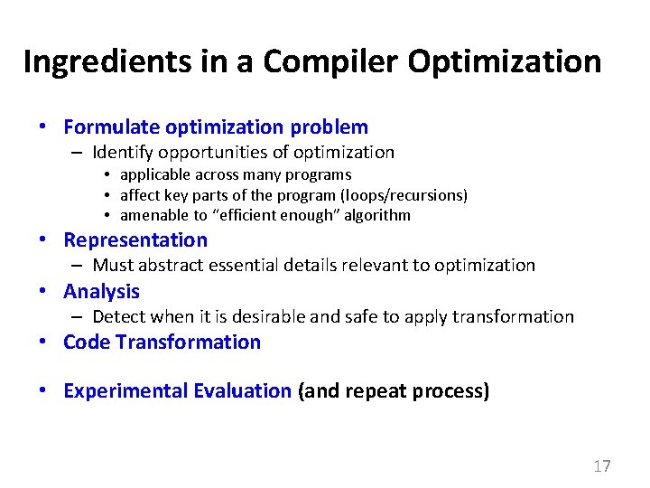
Ingredients in a Compiler Optimization • Formulate optimization problem – Identify opportunities of optimization • applicable across many programs • affect key parts of the program (loops/recursions) • amenable to “efficient enough” algorithm • Representation – Must abstract essential details relevant to optimization • Analysis – Detect when it is desirable and safe to apply transformation • Code Transformation • Experimental Evaluation (and repeat process) 17

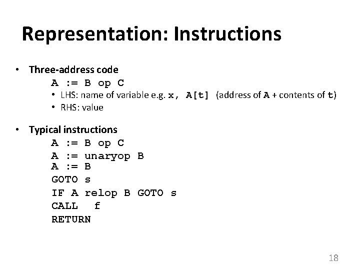
Representation: Instructions • Three-address code A : = B op C • LHS: name of variable e. g. x, A[t] (address of A + contents of t) • RHS: value • Typical instructions A : = B op C A : = unaryop B A : = B GOTO s IF A relop B GOTO s CALL f RETURN 18

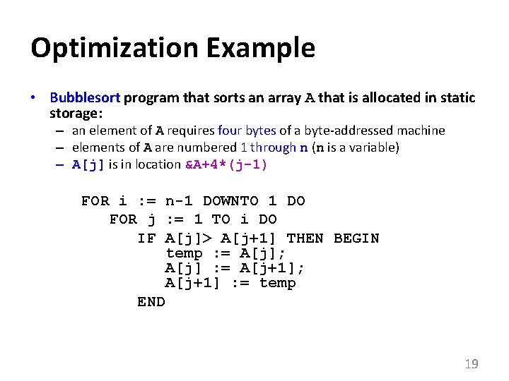
Optimization Example • Bubblesort program that sorts an array A that is allocated in static storage: – an element of A requires four bytes of a byte-addressed machine – elements of A are numbered 1 through n (n is a variable) – A[j] is in location &A+4*(j-1) FOR i : = n-1 DOWNTO 1 DO FOR j : = 1 TO i DO IF A[j]> A[j+1] THEN BEGIN temp : = A[j]; A[j] : = A[j+1]; A[j+1] : = temp END 19

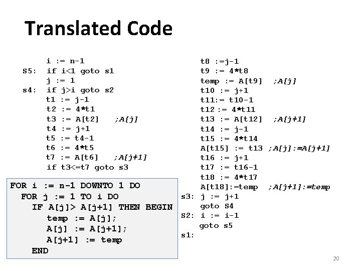
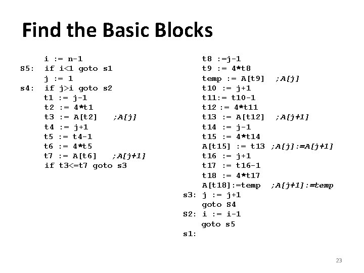
Translated Code S 5: s 4: i : = n-1 if i<1 goto s 1 j : = 1 if j>i goto s 2 t 1 : = j-1 t 2 : = 4*t 1 t 3 : = A[t 2] ; A[j] t 4 : = j+1 t 5 : = t 4 -1 t 6 : = 4*t 5 t 7 : = A[t 6] ; A[j+1] if t 3<=t 7 goto s 3 FOR i : = n-1 DOWNTO 1 DO FOR j : = 1 TO i DO IF A[j]> A[j+1] THEN BEGIN temp : = A[j]; A[j] : = A[j+1]; A[j+1] : = temp END t 8 : =j-1 t 9 : = 4*t 8 temp : = A[t 9] ; A[j] t 10 : = j+1 t 11: = t 10 -1 t 12 : = 4*t 11 t 13 : = A[t 12] ; A[j+1] t 14 : = j-1 t 15 : = 4*t 14 A[t 15] : = t 13 ; A[j]: =A[j+1] t 16 : = j+1 t 17 : = t 16 -1 t 18 : = 4*t 17 A[t 18]: =temp ; A[j+1]: =temp s 3: j : = j+1 goto S 4 S 2: i : = i-1 goto s 5 s 1: 20

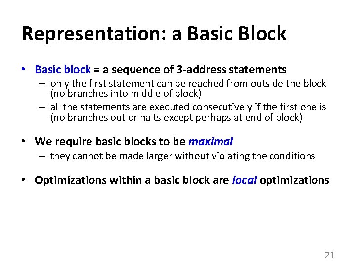
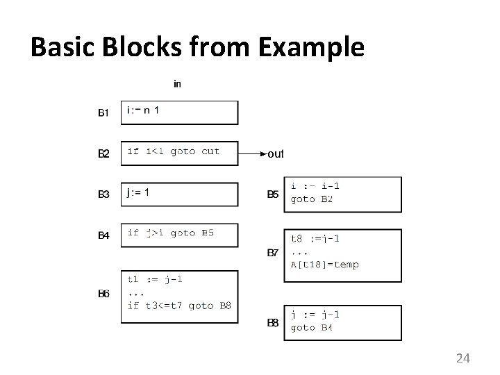
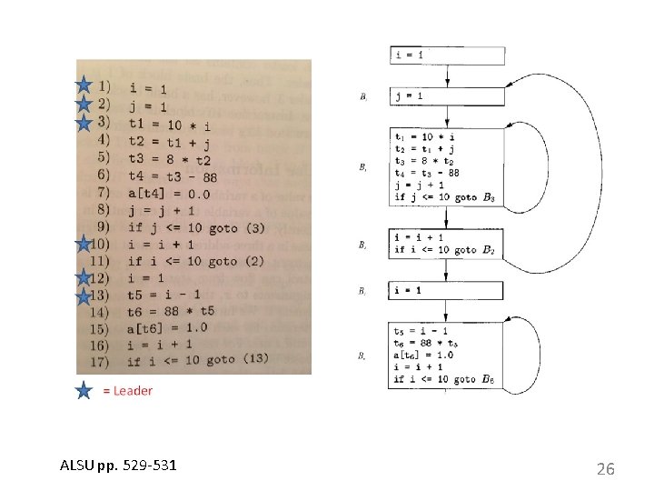
Representation: a Basic Block • Basic block = a sequence of 3 -address statements – only the first statement can be reached from outside the block (no branches into middle of block) – all the statements are executed consecutively if the first one is (no branches out or halts except perhaps at end of block) • We require basic blocks to be maximal – they cannot be made larger without violating the conditions • Optimizations within a basic block are local optimizations 21

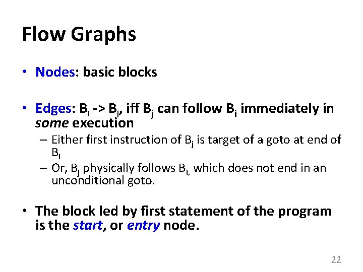
Flow Graphs • Nodes: basic blocks • Edges: Bi -> Bj, iff Bj can follow Bi immediately in some execution – Either first instruction of Bj is target of a goto at end of Bi – Or, Bj physically follows Bi, which does not end in an unconditional goto. • The block led by first statement of the program is the start, or entry node. 22

Find the Basic Blocks S 5: s 4: i : = n-1 if i<1 goto s 1 j : = 1 if j>i goto s 2 t 1 : = j-1 t 2 : = 4*t 1 t 3 : = A[t 2] ; A[j] t 4 : = j+1 t 5 : = t 4 -1 t 6 : = 4*t 5 t 7 : = A[t 6] ; A[j+1] if t 3<=t 7 goto s 3 t 8 : =j-1 t 9 : = 4*t 8 temp : = A[t 9] ; A[j] t 10 : = j+1 t 11: = t 10 -1 t 12 : = 4*t 11 t 13 : = A[t 12] ; A[j+1] t 14 : = j-1 t 15 : = 4*t 14 A[t 15] : = t 13 ; A[j]: =A[j+1] t 16 : = j+1 t 17 : = t 16 -1 t 18 : = 4*t 17 A[t 18]: =temp ; A[j+1]: =temp s 3: j : = j+1 goto S 4 S 2: i : = i-1 goto s 5 s 1: 23

Basic Blocks from Example 24

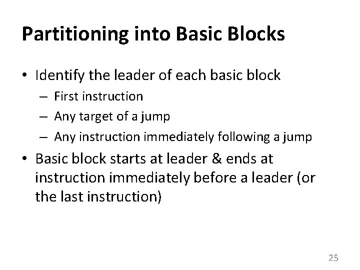
Partitioning into Basic Blocks • Identify the leader of each basic block – First instruction – Any target of a jump – Any instruction immediately following a jump • Basic block starts at leader & ends at instruction immediately before a leader (or the last instruction) 25

ALSU pp. 529 -531 26

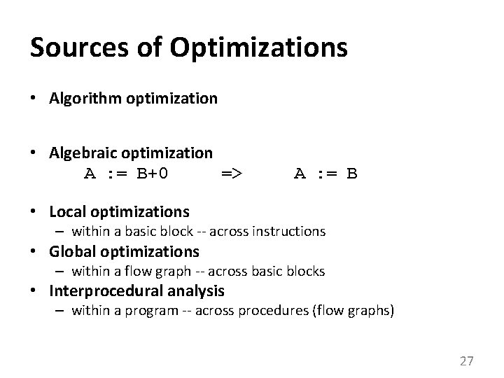
Sources of Optimizations • Algorithm optimization • Algebraic optimization A : = B+0 => A : = B • Local optimizations – within a basic block -- across instructions • Global optimizations – within a flow graph -- across basic blocks • Interprocedural analysis – within a program -- across procedures (flow graphs) 27

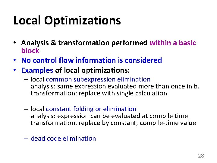
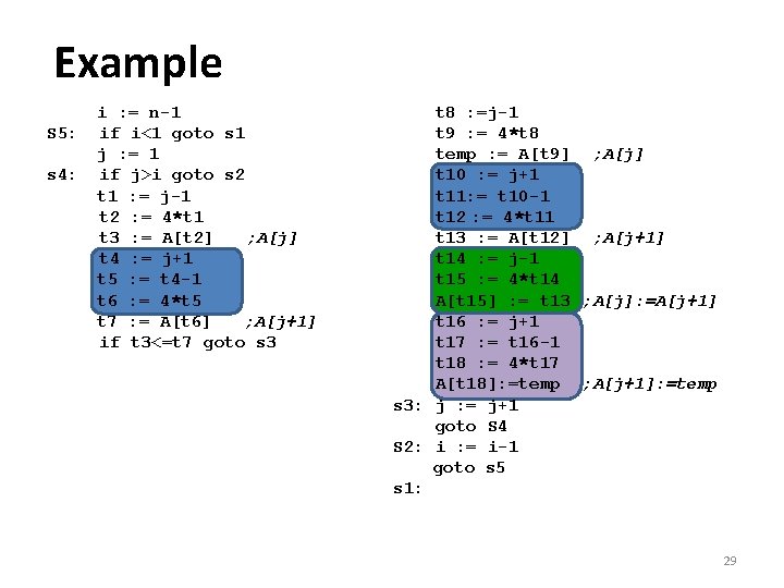
Local Optimizations • Analysis & transformation performed within a basic block • No control flow information is considered • Examples of local optimizations: – local common subexpression elimination analysis: same expression evaluated more than once in b. transformation: replace with single calculation – local constant folding or elimination analysis: expression can be evaluated at compile time transformation: replace by constant, compile-time value – dead code elimination 28

Example S 5: s 4: i : = n-1 if i<1 goto s 1 j : = 1 if j>i goto s 2 t 1 : = j-1 t 2 : = 4*t 1 t 3 : = A[t 2] ; A[j] t 4 : = j+1 t 5 : = t 4 -1 t 6 : = 4*t 5 t 7 : = A[t 6] ; A[j+1] if t 3<=t 7 goto s 3 t 8 : =j-1 t 9 : = 4*t 8 temp : = A[t 9] ; A[j] t 10 : = j+1 t 11: = t 10 -1 t 12 : = 4*t 11 t 13 : = A[t 12] ; A[j+1] t 14 : = j-1 t 15 : = 4*t 14 A[t 15] : = t 13 ; A[j]: =A[j+1] t 16 : = j+1 t 17 : = t 16 -1 t 18 : = 4*t 17 A[t 18]: =temp ; A[j+1]: =temp s 3: j : = j+1 goto S 4 S 2: i : = i-1 goto s 5 s 1: 29

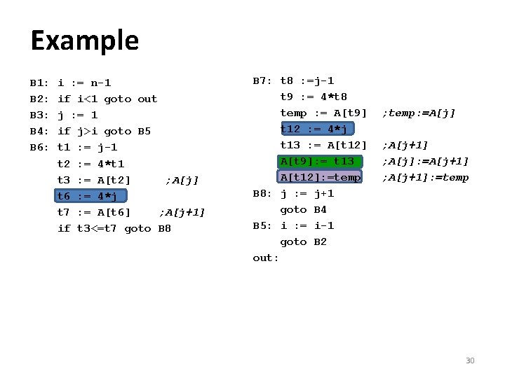
Example B 1: B 2: B 3: B 4: B 6: i : = n-1 if i<1 goto out j : = 1 if j>i goto B 5 t 1 : = j-1 t 2 : = 4*t 1 t 3 : = A[t 2] ; A[j] t 6 : = 4*j t 7 : = A[t 6] ; A[j+1] if t 3<=t 7 goto B 8 B 7: t 8 : =j-1 t 9 : = 4*t 8 temp : = A[t 9] t 12 : = 4*j t 13 : = A[t 12] A[t 9]: = t 13 A[t 12]: =temp B 8: j : = j+1 goto B 4 B 5: i : = i-1 goto B 2 out: ; temp: =A[j] ; A[j+1] ; A[j]: =A[j+1] ; A[j+1]: =temp 30

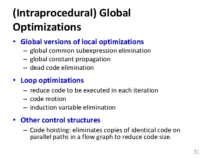
(Intraprocedural) Global Optimizations • Global versions of local optimizations – global common subexpression elimination – global constant propagation – dead code elimination • Loop optimizations – reduce code to be executed in each iteration – code motion – induction variable elimination • Other control structures – Code hoisting: eliminates copies of identical code on parallel paths in a flow graph to reduce code size. 31

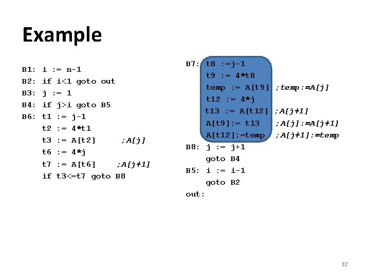
Example B 1: B 2: B 3: B 4: B 6: i : = n-1 if i<1 goto out j : = 1 if j>i goto B 5 t 1 : = j-1 t 2 : = 4*t 1 t 3 : = A[t 2] ; A[j] t 6 : = 4*j t 7 : = A[t 6] ; A[j+1] if t 3<=t 7 goto B 8 B 7: t 8 : =j-1 t 9 : = 4*t 8 temp : = A[t 9] t 12 : = 4*j t 13 : = A[t 12] A[t 9]: = t 13 A[t 12]: =temp B 8: j : = j+1 goto B 4 B 5: i : = i-1 goto B 2 out: ; temp: =A[j] ; A[j+1] ; A[j]: =A[j+1] ; A[j+1]: =temp 32

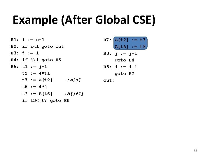
Example (After Global CSE) B 1: B 2: B 3: B 4: B 6: i : = n-1 if i<1 goto out j : = 1 if j>i goto B 5 t 1 : = j-1 t 2 : = 4*t 1 t 3 : = A[t 2] ; A[j] t 6 : = 4*j t 7 : = A[t 6] ; A[j+1] if t 3<=t 7 goto B 8 B 7: A[t 2] : = t 7 A[t 6] : = t 3 B 8: j : = j+1 goto B 4 B 5: i : = i-1 goto B 2 out: 33

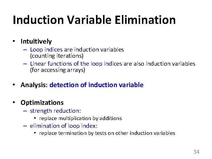
Induction Variable Elimination • Intuitively – Loop indices are induction variables (counting iterations) – Linear functions of the loop indices are also induction variables (for accessing arrays) • Analysis: detection of induction variable • Optimizations – strength reduction: • replace multiplication by additions – elimination of loop index: • replace termination by tests on other induction variables 34

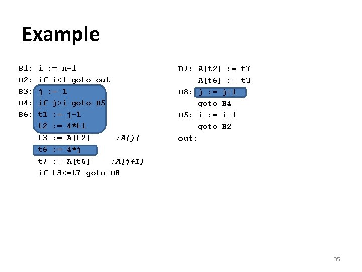
Example B 1: B 2: B 3: B 4: B 6: i : = n-1 if i<1 goto out j : = 1 if j>i goto B 5 t 1 : = j-1 t 2 : = 4*t 1 t 3 : = A[t 2] ; A[j] t 6 : = 4*j t 7 : = A[t 6] ; A[j+1] if t 3<=t 7 goto B 8 B 7: A[t 2] : = t 7 A[t 6] : = t 3 B 8: j : = j+1 goto B 4 B 5: i : = i-1 goto B 2 out: 35

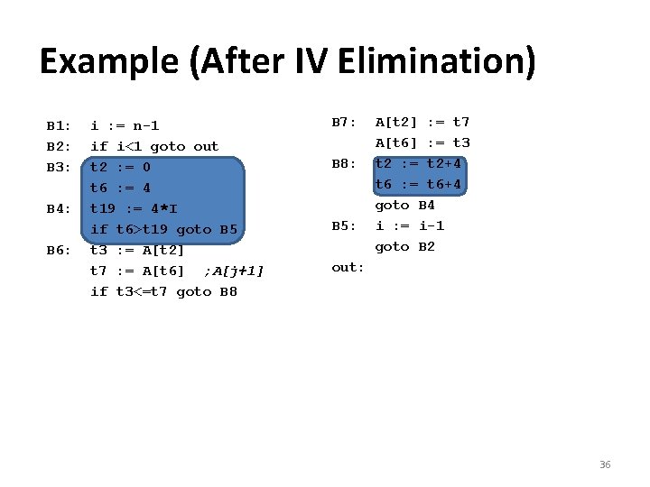
Example (After IV Elimination) B 1: B 2: B 3: B 4: B 6: i : = n-1 if i<1 goto out t 2 : = 0 t 6 : = 4 t 19 : = 4*I if t 6>t 19 goto B 5 t 3 : = A[t 2] t 7 : = A[t 6] ; A[j+1] if t 3<=t 7 goto B 8 B 7: B 8: B 5: A[t 2] : = t 7 A[t 6] : = t 3 t 2 : = t 2+4 t 6 : = t 6+4 goto B 4 i : = i-1 goto B 2 out: 36

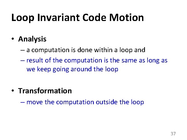
Loop Invariant Code Motion • Analysis – a computation is done within a loop and – result of the computation is the same as long as we keep going around the loop • Transformation – move the computation outside the loop 37

Machine Dependent Optimizations • • Register allocation Instruction scheduling Memory hierarchy optimizations etc. 38

Local Optimizations (More Details) • Common subexpression elimination – array expressions – field access in records – access to parameters 39

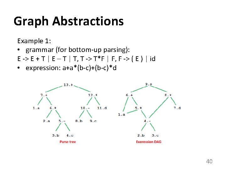
Graph Abstractions Example 1: • grammar (for bottom-up parsing): E -> E + T | E – T | T, T -> T*F | F, F -> ( E ) | id • expression: a+a*(b-c)+(b-c)*d 40

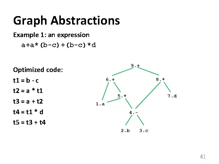
Graph Abstractions Example 1: an expression a+a*(b-c)+(b-c)*d Optimized code: t 1 = b - c t 2 = a * t 1 t 3 = a + t 2 t 4 = t 1 * d t 5 = t 3 + t 4 41

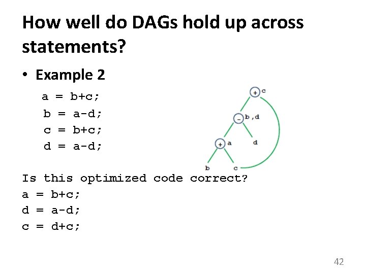
How well do DAGs hold up across statements? • Example 2 a b c d = = b+c; a-d; Is this optimized code correct? a = b+c; d = a-d; c = d+c; 42

Critique of DAGs • Cause of problems – Assignment statements – Value of variable depends on TIME • How to fix problem? – build graph in order of execution – attach variable name to latest value • Final graph created is not very interesting – Key: variable->value mapping across time – loses appeal of abstraction 43

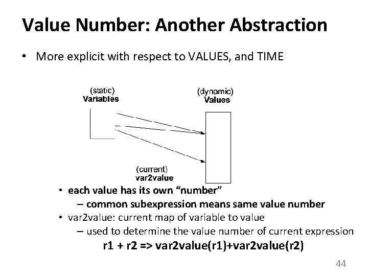
Value Number: Another Abstraction • More explicit with respect to VALUES, and TIME • each value has its own “number” – common subexpression means same value number • var 2 value: current map of variable to value – used to determine the value number of current expression r 1 + r 2 => var 2 value(r 1)+var 2 value(r 2) 44

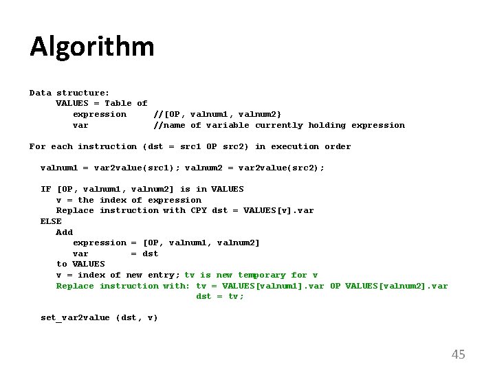
Algorithm Data structure: VALUES = Table of expression //[OP, valnum 1, valnum 2} var //name of variable currently holding expression For each instruction (dst = src 1 OP src 2) in execution order valnum 1 = var 2 value(src 1); valnum 2 = var 2 value(src 2); IF [OP, valnum 1, valnum 2] is in VALUES v = the index of expression Replace instruction with CPY dst = VALUES[v]. var ELSE Add expression = [OP, valnum 1, valnum 2] var = dst to VALUES v = index of new entry; tv is new temporary for v Replace instruction with: tv = VALUES[valnum 1]. var OP VALUES[valnum 2]. var dst = tv; set_var 2 value (dst, v) 45

More Details • What are the initial values of the variables? – values at beginning of the basic block • Possible implementations: – Initialization: create “initial values” for all variables – Or dynamically create them as they are used • Implementation of VALUES and var 2 value: hash tables 46

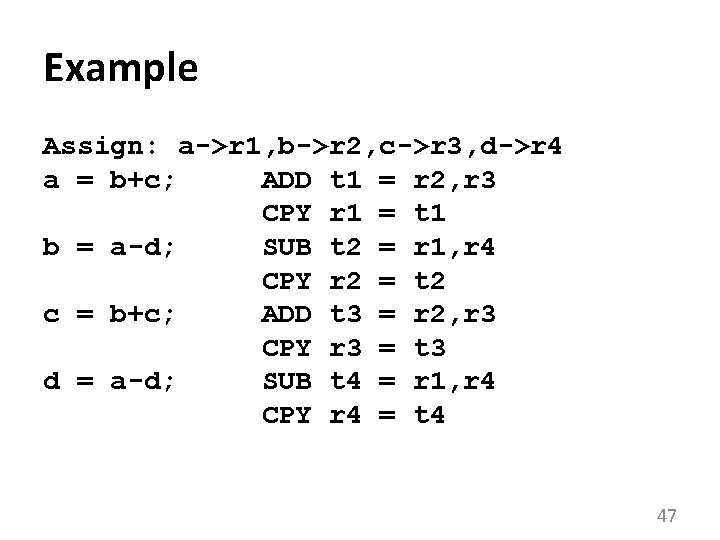
Example Assign: a->r 1, b->r 2, c->r 3, d->r 4 a = b+c; ADD t 1 = r 2, r 3 CPY r 1 = t 1 b = a-d; SUB t 2 = r 1, r 4 CPY r 2 = t 2 c = b+c; ADD t 3 = r 2, r 3 CPY r 3 = t 3 d = a-d; SUB t 4 = r 1, r 4 CPY r 4 = t 4 47

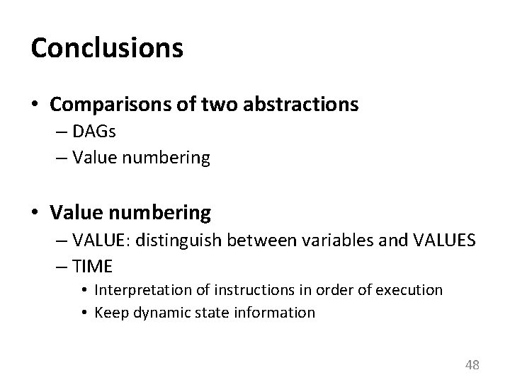
Conclusions • Comparisons of two abstractions – DAGs – Value numbering • Value numbering – VALUE: distinguish between variables and VALUES – TIME • Interpretation of instructions in order of execution • Keep dynamic state information 48

CSC D 70: Compiler Optimization Introduction, Logistics Prof. Gennady Pekhimenko University of Toronto Winter 2018 The content of this lecture is adapted from the lectures of Todd Mowry and Phillip Gibbons