CSC D 70 Compiler Optimization Memory Optimizations Prof

CSC D 70: Compiler Optimization Memory Optimizations Prof. Gennady Pekhimenko University of Toronto Winter 2019 The content of this lecture is adapted from the lectures of Todd Mowry, Greg Steffan, and Phillip Gibbons

Pointer Analysis (Summary) • Pointers are hard to understand at compile time! – accurate analyses are large and complex • Many different options: – Representation, heap modeling, aggregate modeling, flow sensitivity, context sensitivity • Many algorithms: – Address-taken, Steensgarde, Andersen – BDD-based, probabilistic • Many trade-offs: – space, time, accuracy, safety • Choose the right type of analysis given how the information will be used 2

Caches: A Quick Review • How do they work? • Why do we care about them? • What are typical configurations today? • What are some important cache parameters that will affect performance? 3

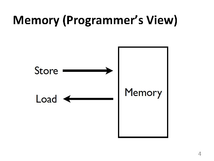
Memory (Programmer’s View) 4

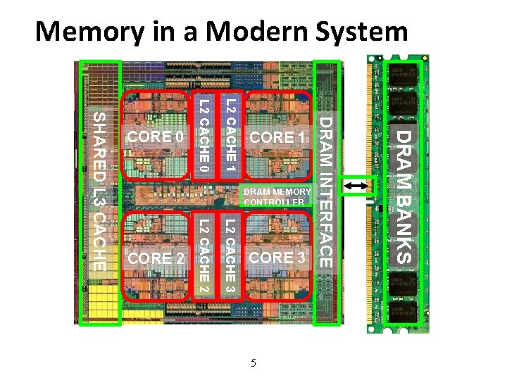
Memory in a Modern System 5 DRAM BANKS L 2 CACHE 3 L 2 CACHE 2 SHARED L 3 CACHE DRAM MEMORY CONTROLLER DRAM INTERFACE L 2 CACHE 1 L 2 CACHE 0 CORE 3 CORE 2 CORE 1 CORE 0

Ideal Memory • • Zero access time (latency) Infinite capacity Zero cost Infinite bandwidth (to support multiple accesses in parallel) 6

The Problem • Ideal memory’s requirements oppose each other • Bigger is slower – Bigger Takes longer to determine the location • Faster is more expensive – Memory technology: SRAM vs. DRAM vs. Flash vs. Disk vs. Tape • Higher bandwidth is more expensive – Need more banks, more ports, higher frequency, or faster technology 7

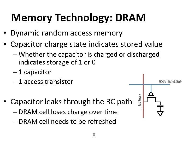
Memory Technology: DRAM • Dynamic random access memory • Capacitor charge state indicates stored value • Capacitor leaks through the RC path – DRAM cell loses charge over time – DRAM cell needs to be refreshed 8 _bitline – Whether the capacitor is charged or discharged indicates storage of 1 or 0 – 1 capacitor row enable – 1 access transistor

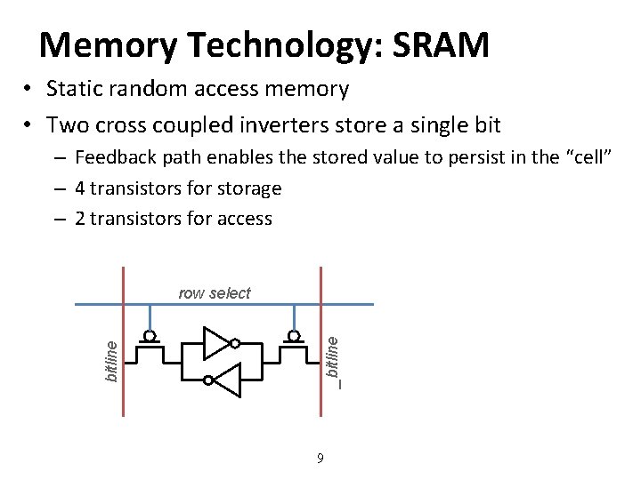
Memory Technology: SRAM • Static random access memory • Two cross coupled inverters store a single bit – Feedback path enables the stored value to persist in the “cell” – 4 transistors for storage – 2 transistors for access _bitline row select 9

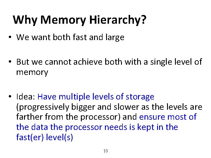
Why Memory Hierarchy? • We want both fast and large • But we cannot achieve both with a single level of memory • Idea: Have multiple levels of storage (progressively bigger and slower as the levels are farther from the processor) and ensure most of the data the processor needs is kept in the fast(er) level(s) 10

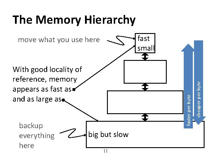
The Memory Hierarchy backup everything here faster per byte With good locality of reference, memory appears as fast as and as large as big but slow 11 cheaper byte fast small move what you use here

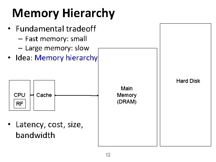
Memory Hierarchy • Fundamental tradeoff – Fast memory: small – Large memory: slow • Idea: Memory hierarchy Hard Disk CPU Main Memory (DRAM) Cache RF • Latency, cost, size, bandwidth 12

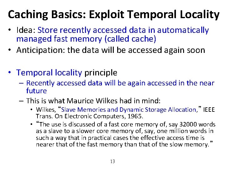
Caching Basics: Exploit Temporal Locality • Idea: Store recently accessed data in automatically managed fast memory (called cache) • Anticipation: the data will be accessed again soon • Temporal locality principle – Recently accessed data will be again accessed in the near future – This is what Maurice Wilkes had in mind: • Wilkes, “Slave Memories and Dynamic Storage Allocation, ” IEEE Trans. On Electronic Computers, 1965. • “The use is discussed of a fast core memory of, say 32000 words as a slave to a slower core memory of, say, one million words in such a way that in practical cases the effective access time is nearer that of the fast memory than that of the slow memory. ” 13

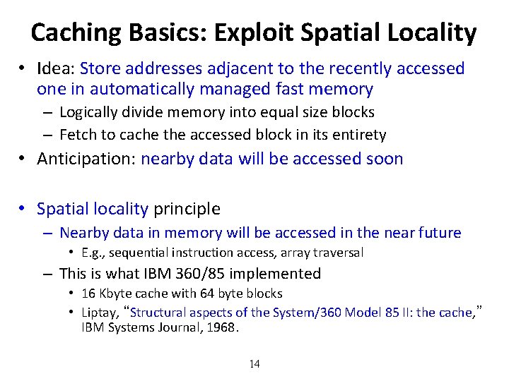
Caching Basics: Exploit Spatial Locality • Idea: Store addresses adjacent to the recently accessed one in automatically managed fast memory – Logically divide memory into equal size blocks – Fetch to cache the accessed block in its entirety • Anticipation: nearby data will be accessed soon • Spatial locality principle – Nearby data in memory will be accessed in the near future • E. g. , sequential instruction access, array traversal – This is what IBM 360/85 implemented • 16 Kbyte cache with 64 byte blocks • Liptay, “Structural aspects of the System/360 Model 85 II: the cache, ” IBM Systems Journal, 1968. 14

Optimizing Cache Performance • Things to enhance: – temporal locality – spatial locality • Things to minimize: – conflicts (i. e. bad replacement decisions) What can the compiler do to help? 15

Two Things We Can Manipulate • Time: – When is an object accessed? • Space: – Where does an object exist in the address space? How do we exploit these two levers? 16

Time: Reordering Computation • What makes it difficult to know when an object is accessed? • How can we predict a better time to access it? – What information is needed? • How do we know that this would be safe? 17

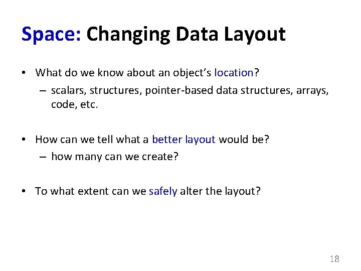
Space: Changing Data Layout • What do we know about an object’s location? – scalars, structures, pointer-based data structures, arrays, code, etc. • How can we tell what a better layout would be? – how many can we create? • To what extent can we safely alter the layout? 18

Types of Objects to Consider • Scalars • Structures & Pointers • Arrays 19

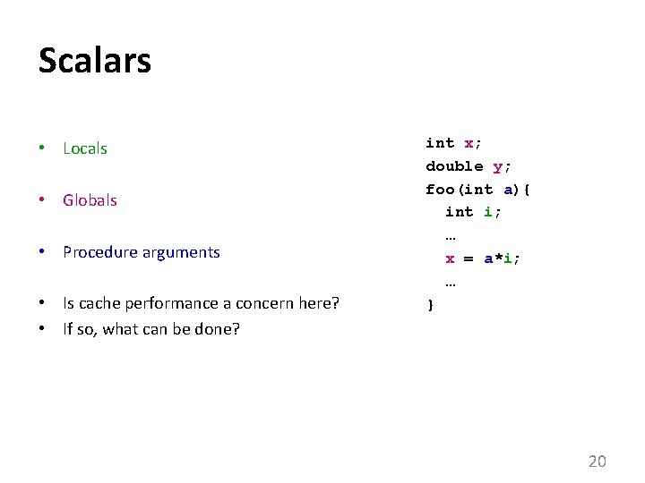
Scalars • Locals • Globals • Procedure arguments • Is cache performance a concern here? • If so, what can be done? int x; double y; foo(int a){ int i; … x = a*i; … } 20

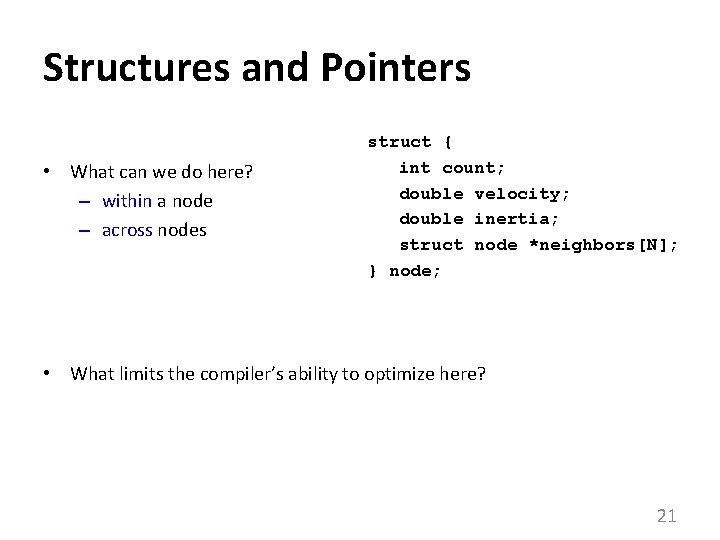
Structures and Pointers • What can we do here? – within a node – across nodes struct { int count; double velocity; double inertia; struct node *neighbors[N]; } node; • What limits the compiler’s ability to optimize here? 21

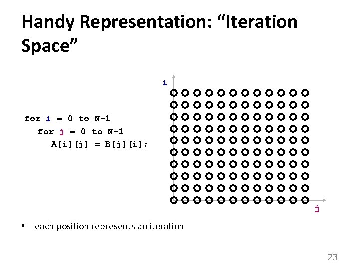
Arrays double A[N][N], B[N][N]; … for i = 0 to N-1 for j = 0 to N-1 A[i][j] = B[j][i]; • usually accessed within loops nests – makes it easy to understand “time” • what we know about array element addresses: – start of array? – relative position within array 22

Handy Representation: “Iteration Space” i for i = 0 to N-1 for j = 0 to N-1 A[i][j] = B[j][i]; j • each position represents an iteration 23

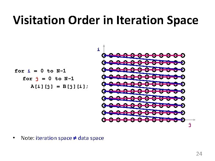
Visitation Order in Iteration Space i for i = 0 to N-1 for j = 0 to N-1 A[i][j] = B[j][i]; j • Note: iteration space data space 24

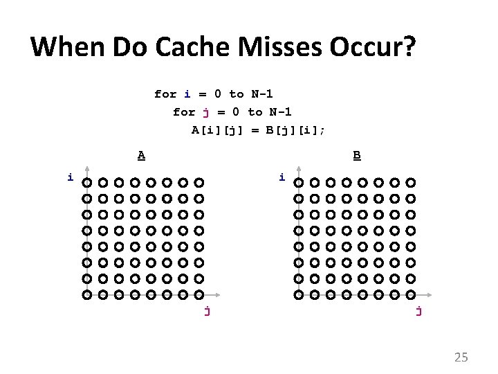
When Do Cache Misses Occur? for i = 0 to N-1 for j = 0 to N-1 A[i][j] = B[j][i]; A B i i j j 25

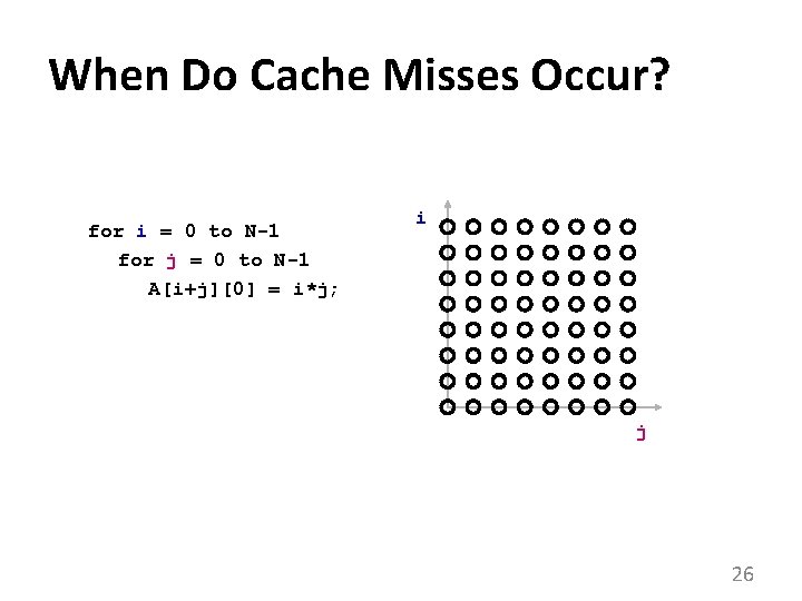
When Do Cache Misses Occur? for i = 0 to N-1 for j = 0 to N-1 A[i+j][0] = i*j; i j 26

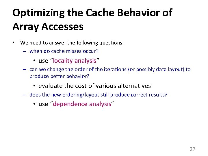
Optimizing the Cache Behavior of Array Accesses • We need to answer the following questions: – when do cache misses occur? • use “locality analysis” – can we change the order of the iterations (or possibly data layout) to produce better behavior? • evaluate the cost of various alternatives – does the new ordering/layout still produce correct results? • use “dependence analysis” 27

Examples of Loop Transformations • • • Loop Interchange Cache Blocking Skewing Loop Reversal … 28

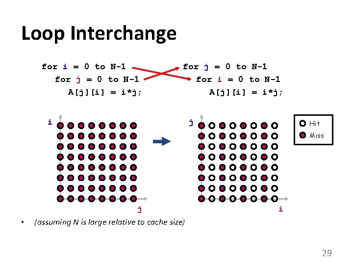
Loop Interchange for i = 0 to N-1 for j = 0 to N-1 A[j][i] = i*j; for j = 0 to N-1 for i = 0 to N-1 A[j][i] = i*j; i j Hit Miss j • i (assuming N is large relative to cache size) 29

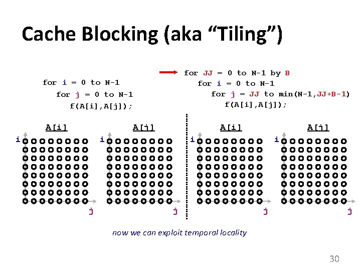
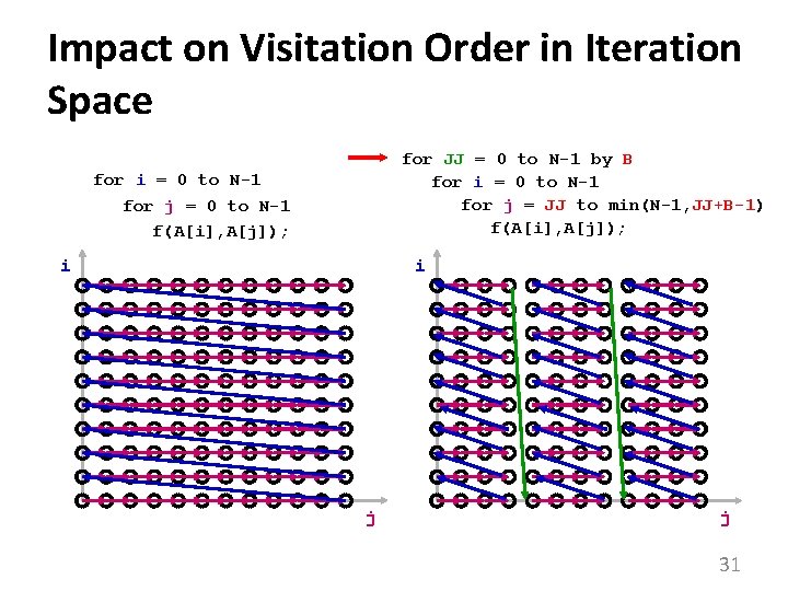
Cache Blocking (aka “Tiling”) for JJ = 0 to N-1 by B for i = 0 to N-1 for j = JJ to min(N-1, JJ+B-1) f(A[i], A[j]); for i = 0 to N-1 for j = 0 to N-1 f(A[i], A[j]); A[i] A[j] i A[i] i j A[j] i j j now we can exploit temporal locality 30

Impact on Visitation Order in Iteration Space for JJ = 0 to N-1 by B for i = 0 to N-1 for j = JJ to min(N-1, JJ+B-1) f(A[i], A[j]); for i = 0 to N-1 for j = 0 to N-1 f(A[i], A[j]); i i j j 31

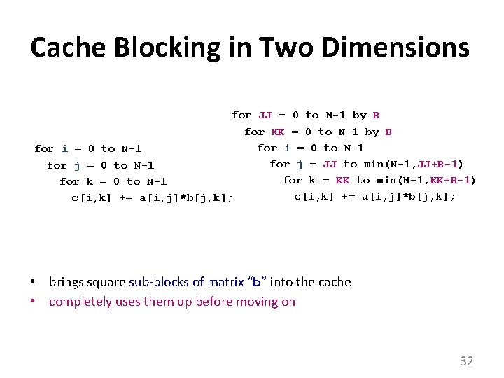
Cache Blocking in Two Dimensions for JJ = 0 to N-1 by B for KK = 0 to N-1 by B for i = 0 to N-1 for j = JJ to min(N-1, JJ+B-1) for j = 0 to N-1 for k = KK to min(N-1, KK+B-1) for k = 0 to N-1 c[i, k] += a[i, j]*b[j, k]; • brings square sub-blocks of matrix “b” into the cache • completely uses them up before moving on 32

Predicting Cache Behavior through “Locality Analysis” • Definitions: – Reuse: • accessing a location that has been accessed in the past – Locality: • accessing a location that is now found in the cache • Key Insights – Locality only occurs when there is reuse! – BUT, reuse does not necessarily result in locality. • why not? 33

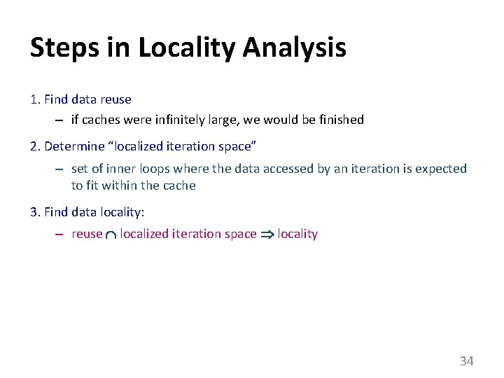
Steps in Locality Analysis 1. Find data reuse – if caches were infinitely large, we would be finished 2. Determine “localized iteration space” – set of inner loops where the data accessed by an iteration is expected to fit within the cache 3. Find data locality: – reuse localized iteration space locality 34

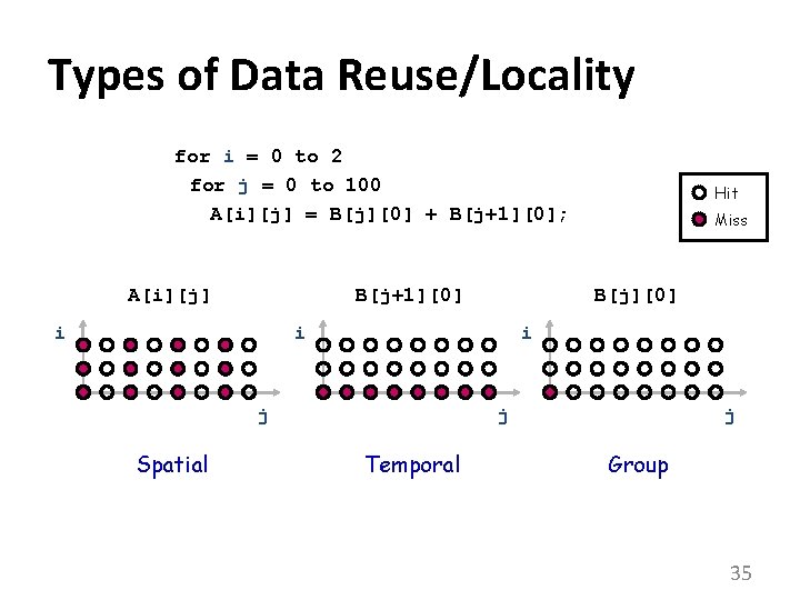
Types of Data Reuse/Locality for i = 0 to 2 for j = 0 to 100 A[i][j] = B[j][0] + B[j+1][0]; A[i][j] B[j+1][0] i Miss B[j][0] i i j Spatial Hit j Temporal j Group 35

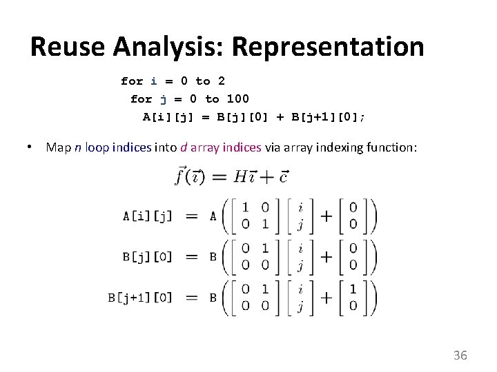
Reuse Analysis: Representation for i = 0 to 2 for j = 0 to 100 A[i][j] = B[j][0] + B[j+1][0]; • Map n loop indices into d array indices via array indexing function: 36

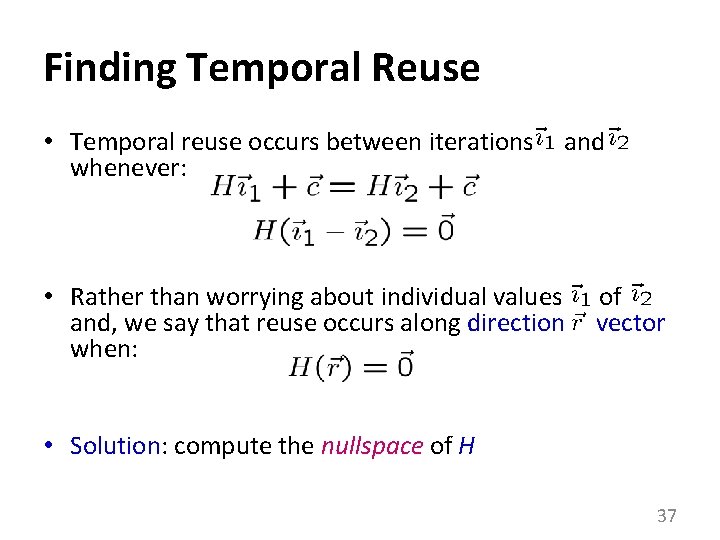
Finding Temporal Reuse • Temporal reuse occurs between iterations whenever: and • Rather than worrying about individual values and, we say that reuse occurs along direction when: of vector • Solution: compute the nullspace of H 37

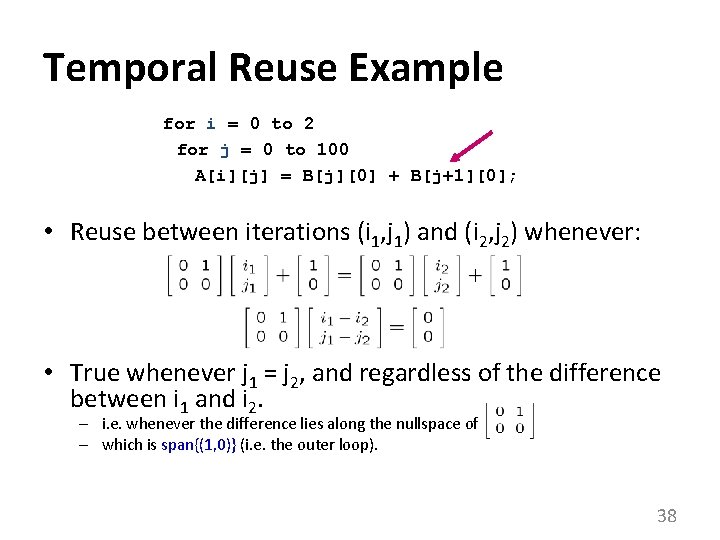
Temporal Reuse Example for i = 0 to 2 for j = 0 to 100 A[i][j] = B[j][0] + B[j+1][0]; • Reuse between iterations (i 1, j 1) and (i 2, j 2) whenever: • True whenever j 1 = j 2, and regardless of the difference between i 1 and i 2. – i. e. whenever the difference lies along the nullspace of – which is span{(1, 0)} (i. e. the outer loop). , 38

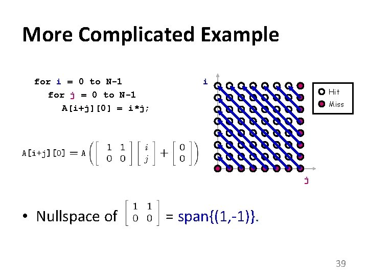
More Complicated Example for i = 0 to N-1 for j = 0 to N-1 A[i+j][0] = i*j; i Hit Miss j • Nullspace of = span{(1, -1)}. 39

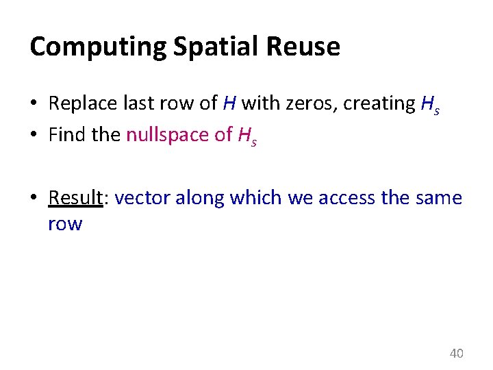
Computing Spatial Reuse • Replace last row of H with zeros, creating Hs • Find the nullspace of Hs • Result: vector along which we access the same row 40

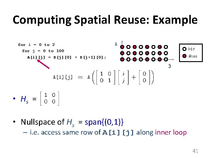
Computing Spatial Reuse: Example for i = 0 to 2 for j = 0 to 100 A[i][j] = B[j][0] + B[j+1][0]; i Hit Miss j • Hs = • Nullspace of Hs = span{(0, 1)} – i. e. access same row of A[i][j] along inner loop 41

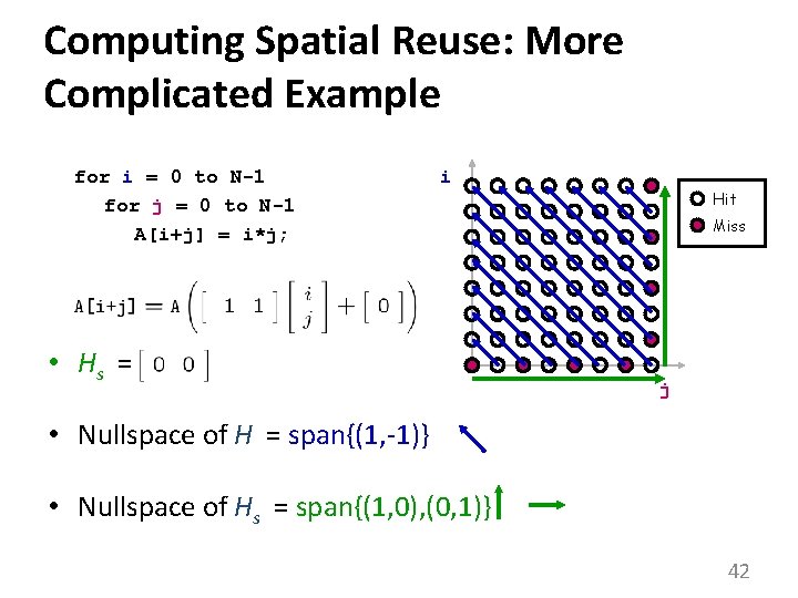
Computing Spatial Reuse: More Complicated Example for i = 0 to N-1 for j = 0 to N-1 A[i+j] = i*j; i • Hs = Hit Miss j • Nullspace of H = span{(1, -1)} • Nullspace of Hs = span{(1, 0), (0, 1)} 42

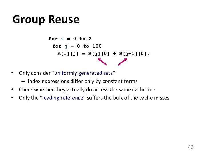
Group Reuse for i = 0 to 2 for j = 0 to 100 A[i][j] = B[j][0] + B[j+1][0]; • Only consider “uniformly generated sets” – index expressions differ only by constant terms • Check whether they actually do access the same cache line • Only the “leading reference” suffers the bulk of the cache misses 43

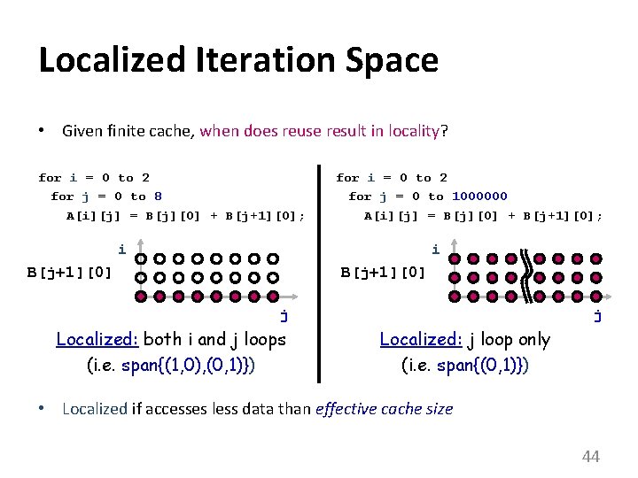
Localized Iteration Space • Given finite cache, when does reuse result in locality? for i = 0 to 2 for j = 0 to 8 A[i][j] = B[j][0] + B[j+1][0]; for i = 0 to 2 for j = 0 to 1000000 A[i][j] = B[j][0] + B[j+1][0]; i i B[j+1][0] j Localized: both i and j loops (i. e. span{(1, 0), (0, 1)}) j Localized: j loop only (i. e. span{(0, 1)}) • Localized if accesses less data than effective cache size 44

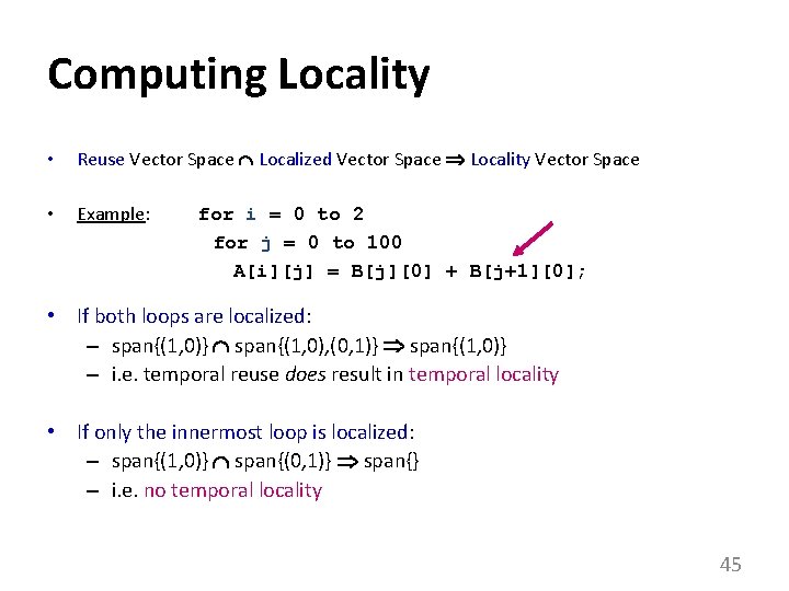
Computing Locality • Reuse Vector Space Localized Vector Space Locality Vector Space • Example: for i = 0 to 2 for j = 0 to 100 A[i][j] = B[j][0] + B[j+1][0]; • If both loops are localized: – span{(1, 0)} span{(1, 0), (0, 1)} span{(1, 0)} – i. e. temporal reuse does result in temporal locality • If only the innermost loop is localized: – span{(1, 0)} span{(0, 1)} span{} – i. e. no temporal locality 45

CSC D 70: Compiler Optimization Memory Optimizations Prof. Gennady Pekhimenko University of Toronto Winter 2019 The content of this lecture is adapted from the lectures of Todd Mowry and Phillip Gibbons