CSC D 70 Compiler Optimization Static Single Assignment

CSC D 70: Compiler Optimization Static Single Assignment (SSA) Prof. Gennady Pekhimenko University of Toronto Winter 2020 The content of this lecture is adapted from the lectures of Todd Mowry and Phillip Gibbons

From Last Lecture • What is a Loop? • Dominator Tree • Natural Loops • Back Edges 2

Finding Loops: Summary • Define loops in graph theoretic terms • Definitions and algorithms for: – Dominators – Back edges – Natural loops 3

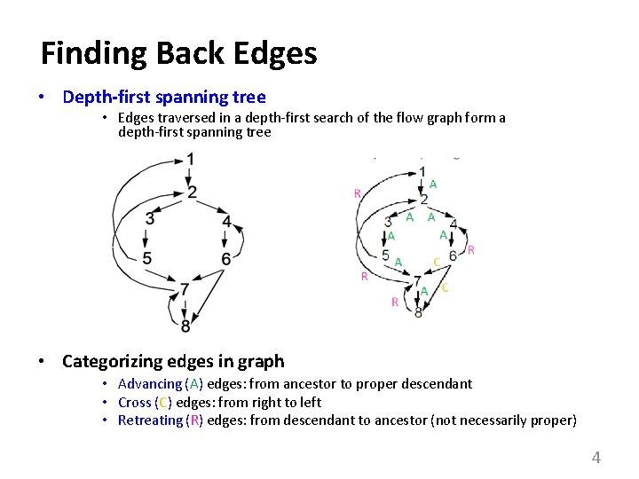
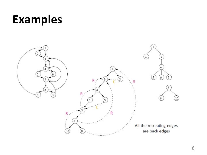
Finding Back Edges • Depth-first spanning tree • Edges traversed in a depth-first search of the flow graph form a depth-first spanning tree • Categorizing edges in graph • Advancing (A) edges: from ancestor to proper descendant • Cross (C) edges: from right to left • Retreating (R) edges: from descendant to ancestor (not necessarily proper) 4

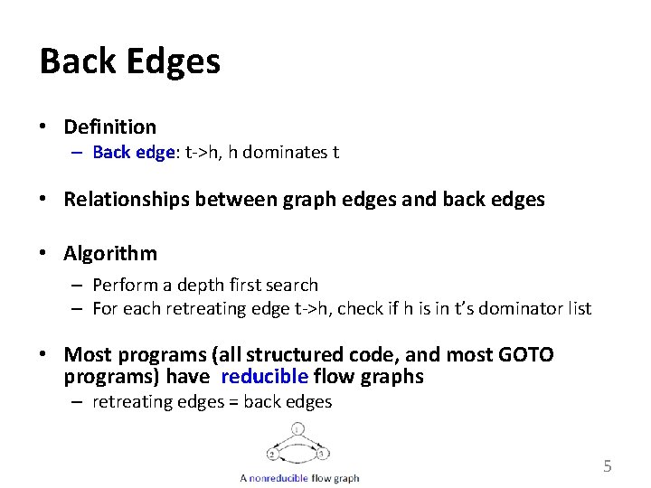
Back Edges • Definition – Back edge: t->h, h dominates t • Relationships between graph edges and back edges • Algorithm – Perform a depth first search – For each retreating edge t->h, check if h is in t’s dominator list • Most programs (all structured code, and most GOTO programs) have reducible flow graphs – retreating edges = back edges 5

Examples 6

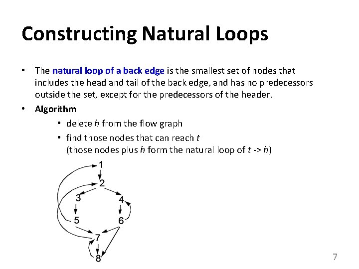
Constructing Natural Loops • The natural loop of a back edge is the smallest set of nodes that includes the head and tail of the back edge, and has no predecessors outside the set, except for the predecessors of the header. • Algorithm • delete h from the flow graph • find those nodes that can reach t (those nodes plus h form the natural loop of t -> h) 7

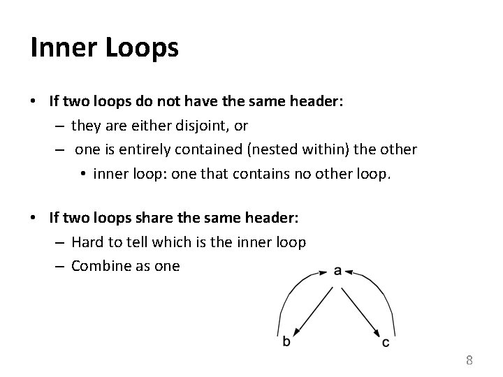
Inner Loops • If two loops do not have the same header: – they are either disjoint, or – one is entirely contained (nested within) the other • inner loop: one that contains no other loop. • If two loops share the same header: – Hard to tell which is the inner loop – Combine as one 8

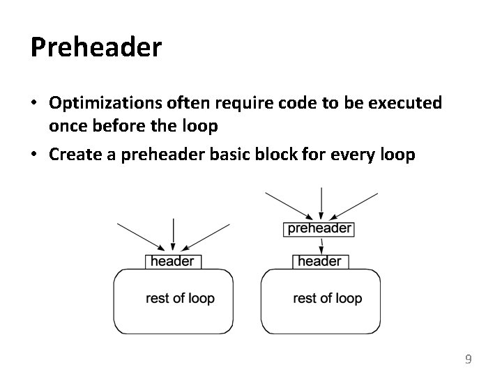
Preheader • Optimizations often require code to be executed once before the loop • Create a preheader basic block for every loop 9

CSC D 70: Compiler Optimization Static Single Assignment (SSA) Prof. Gennady Pekhimenko University of Toronto Winter 2020 The content of this lecture is adapted from the lectures of Todd Mowry and Phillip Gibbons

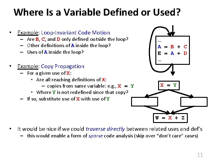
Where Is a Variable Defined or Used? • Example: Loop-Invariant Code Motion – Are B, C, and D only defined outside the loop? – Other definitions of A inside the loop? – Uses of A inside the loop? • Example: Copy Propagation – For a given use of X: • Are all reaching definitions of X: – copies from same variable: e. g. , X = Y • Where Y is not redefined since that copy? – If so, substitute use of X with use of Y X = Y … A = B + C E = A + D … X = Y W = X + Z • It would be nice if we could traverse directly between related uses and def’s – this would enable a form of sparse code analysis (skip over “don’t care” cases) 11

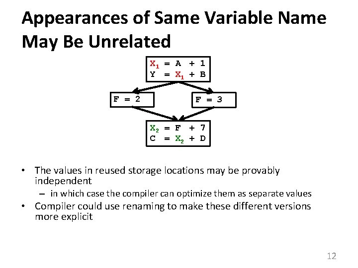
Appearances of Same Variable Name May Be Unrelated X 1 = A 2 + 1 Y 2 = X 1 + B F = 2 F = 3 X 2 = F 2 + 7 C 2 = X 2 + D • The values in reused storage locations may be provably independent – in which case the compiler can optimize them as separate values • Compiler could use renaming to make these different versions more explicit 12

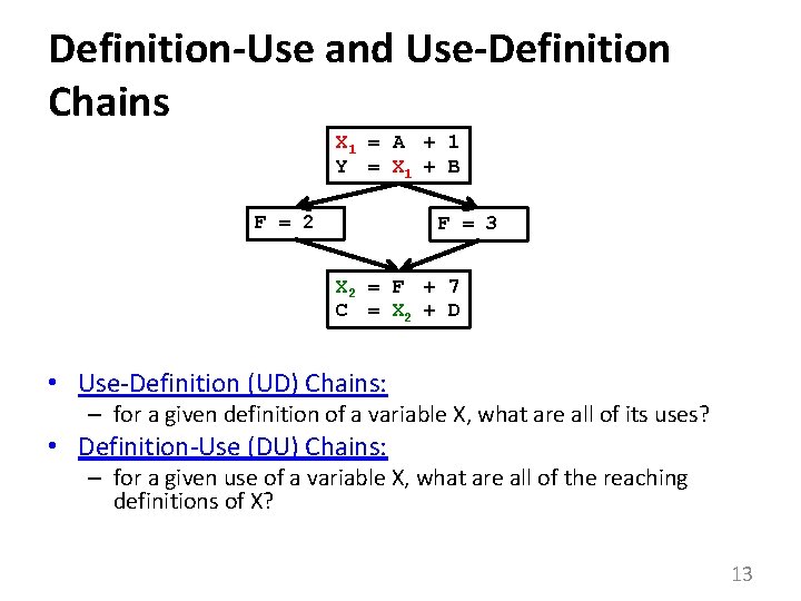
Definition-Use and Use-Definition Chains X 1 = A 2 + 1 Y 2 = X 1 + B F = 2 F = 3 X 2 = F 2 + 7 C 2 = X 2 + D • Use-Definition (UD) Chains: – for a given definition of a variable X, what are all of its uses? • Definition-Use (DU) Chains: – for a given use of a variable X, what are all of the reaching definitions of X? 13

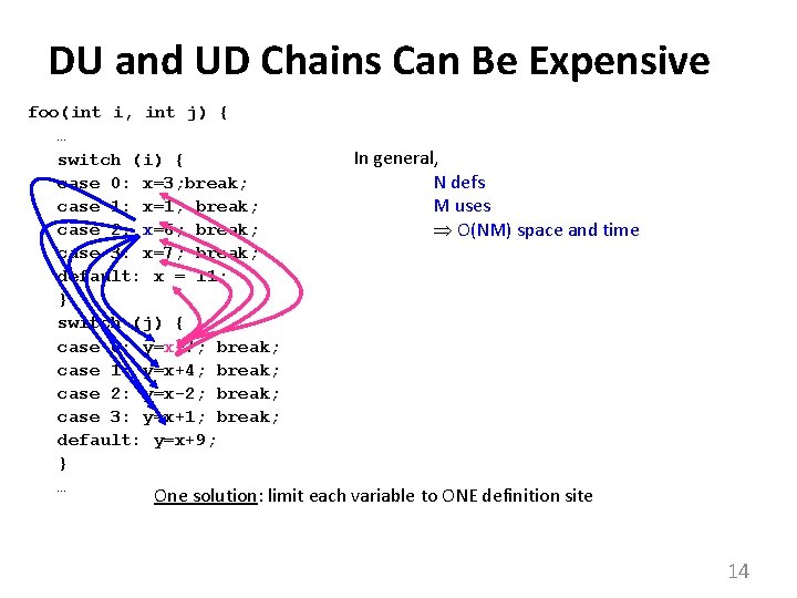
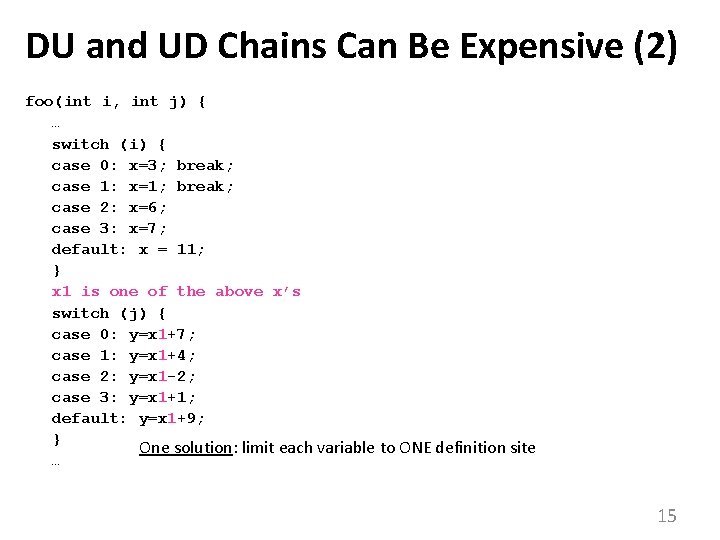
DU and UD Chains Can Be Expensive foo(int i, int j) { … switch (i) { case 0: x=3; break; case 1: x=1; break; case 2: x=6; break; case 3: x=7; break; default: x = 11; } switch (j) { case 0: y=x+7; break; case 1: y=x+4; break; case 2: y=x-2; break; case 3: y=x+1; break; default: y=x+9; } … In general, N defs M uses O(NM) space and time One solution: limit each variable to ONE definition site 14

DU and UD Chains Can Be Expensive (2) foo(int i, int j) { … switch (i) { case 0: x=3; break; case 1: x=1; break; case 2: x=6; case 3: x=7; default: x = 11; } x 1 is one of the above x’s switch (j) { case 0: y=x 1+7; case 1: y=x 1+4; case 2: y=x 1 -2; case 3: y=x 1+1; default: y=x 1+9; } One solution: limit each variable to ONE definition site … 15

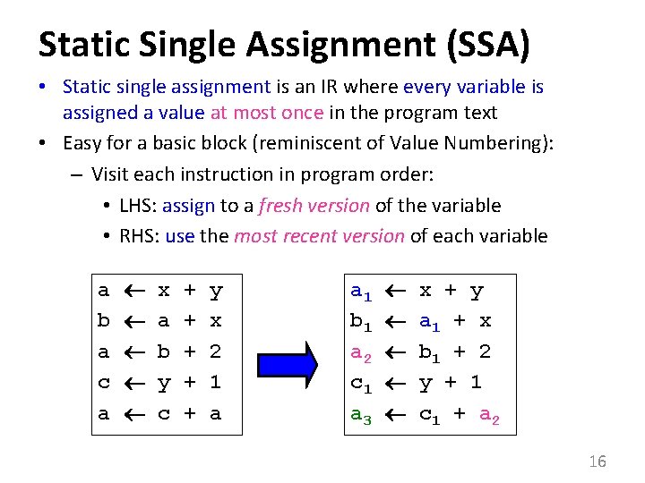
Static Single Assignment (SSA) • Static single assignment is an IR where every variable is assigned a value at most once in the program text • Easy for a basic block (reminiscent of Value Numbering): – Visit each instruction in program order: • LHS: assign to a fresh version of the variable • RHS: use the most recent version of each variable a b a c a x a b y c + + + y x 2 1 a a 1 b 1 a 2 c 1 a 3 x + y a 1 + x b 1 + 2 y + 1 c 1 + a 2 16

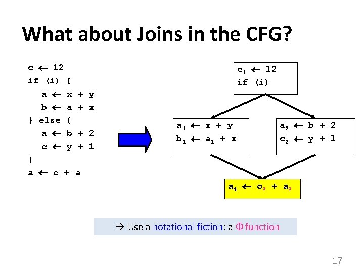
What about Joins in the CFG? c 12 if (i) { a x + b a + } else { a b + c y + } a c + a c 1 12 if (i) y x 2 1 a 1 x + y b 1 a 1 + x a 2 b + 2 c 2 y + 1 a 4 c ? + a ? Use a notational fiction: a function 17

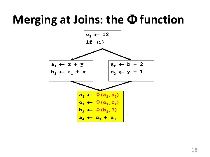
Merging at Joins: the function c 1 12 if (i) a 1 x + y b 1 a 1 + x a 3 c 3 b 2 a 4 a 2 b + 2 c 2 y + 1 (a 1, a 2) (c 1, c 2) (b 1, ? ) c 3 + a 3 18

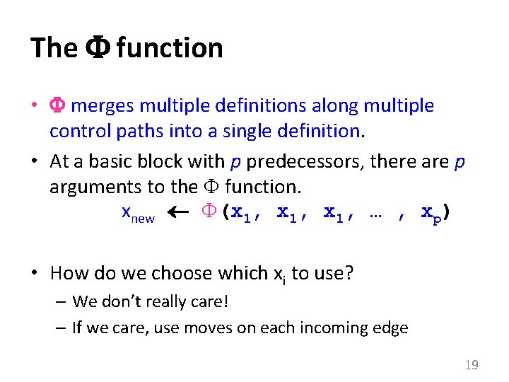
The function • merges multiple definitions along multiple control paths into a single definition. • At a basic block with p predecessors, there are p arguments to the function. xnew (x 1, … , xp) • How do we choose which xi to use? – We don’t really care! – If we care, use moves on each incoming edge 19

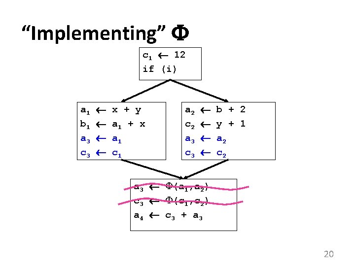
“Implementing” c 1 12 if (i) a 1 b 1 a 3 c 3 x + y a 1 + x a 1 c 1 a 2 c 2 a 3 c 3 b + 2 y + 1 a 2 c 2 a 3 (a 1, a 2) c 3 (c 1, c 2) a 4 c 3 + a 3 20

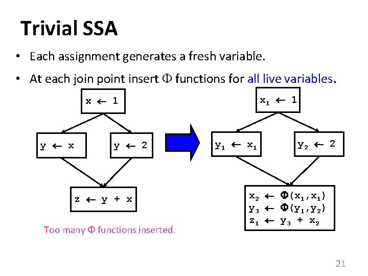
Trivial SSA • Each assignment generates a fresh variable. • At each join point insert functions for all live variables. x 1 1 x 1 y x y 2 z y + x Too many functions inserted. y 1 x 1 y 2 2 x 2 (x 1, x 1) y 3 (y 1, y 2) z 1 y 3 + x 2 21

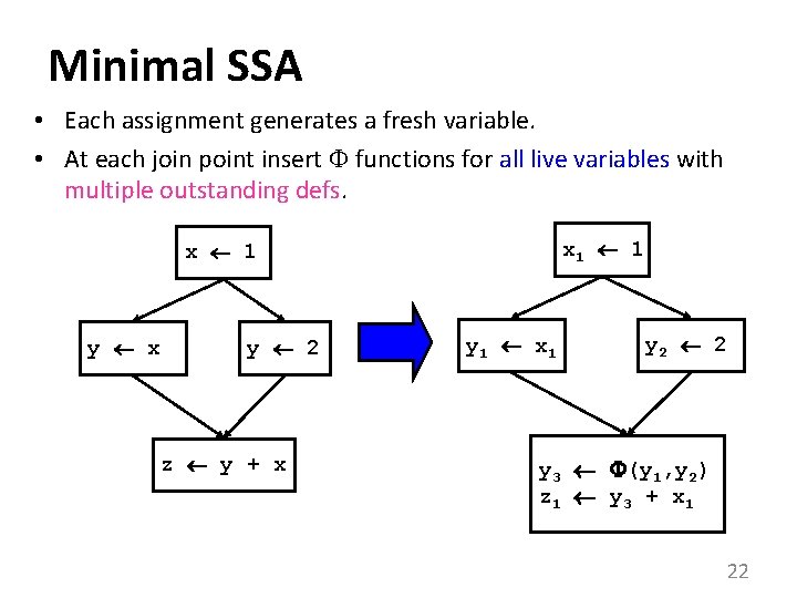
Minimal SSA • Each assignment generates a fresh variable. • At each join point insert functions for all live variables with multiple outstanding defs. x 1 1 x 1 y x y 2 z y + x y 1 x 1 y 2 2 y 3 (y 1, y 2) z 1 y 3 + x 1 22

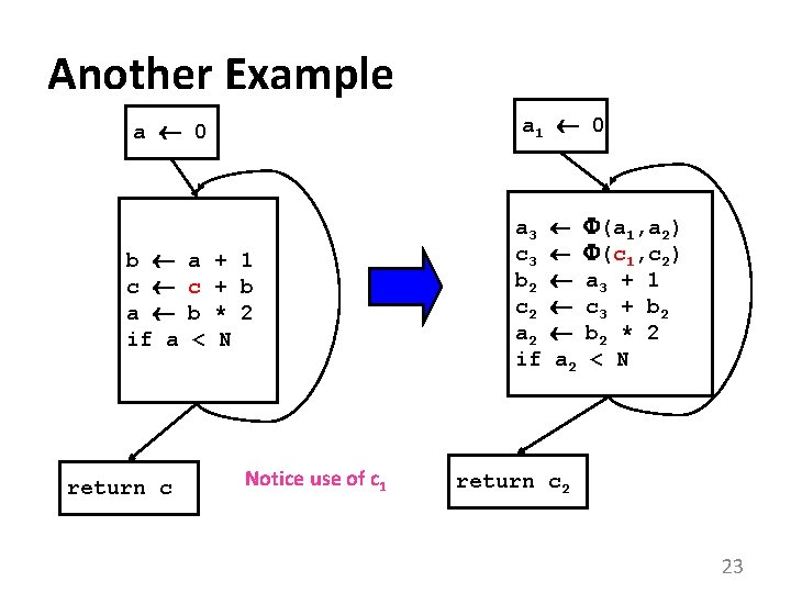
Another Example a 0 a 1 0 b c a if a a 3 c 3 b 2 c 2 a 2 if return c a c b < + 1 + b * 2 N Notice use of c 1 (a 1, a 2) (c 1, c 2) a 2 a 3 c 3 b 2 < + 1 + b 2 * 2 N return c 2 23

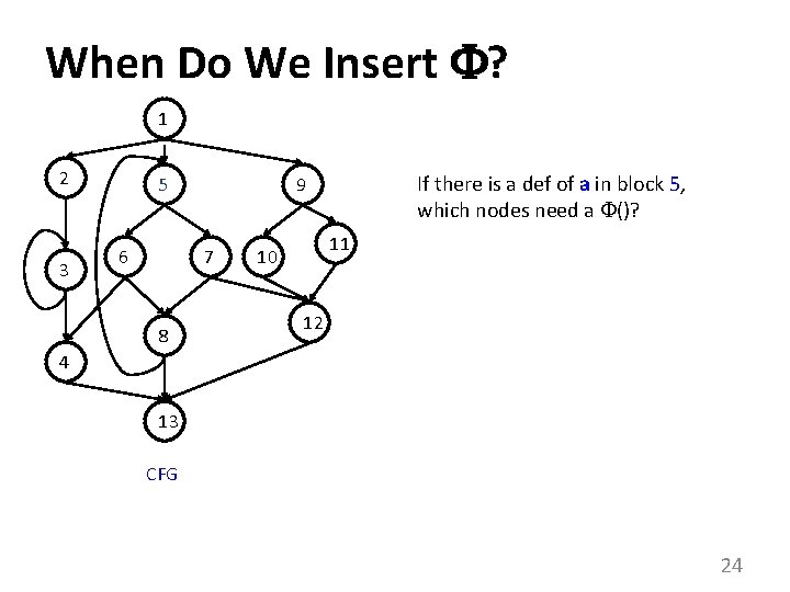
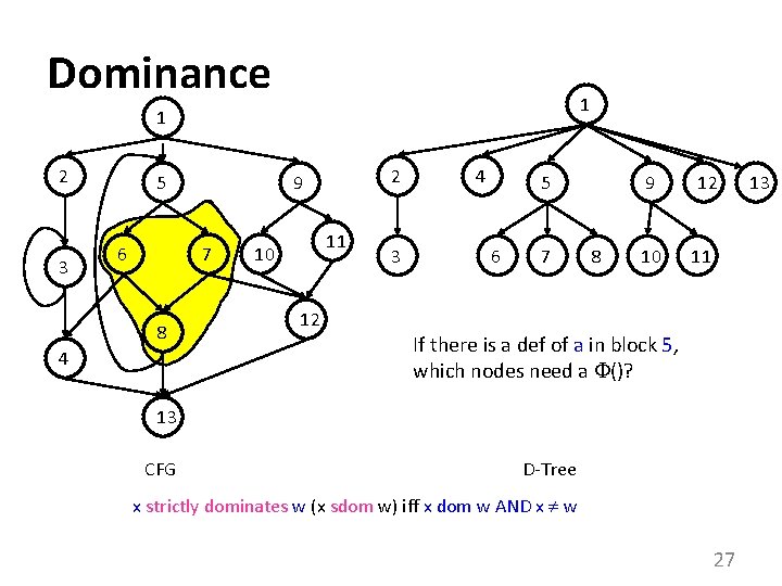
When Do We Insert ? 1 2 3 5 6 7 8 If there is a def of a in block 5, which nodes need a ()? 9 11 10 12 4 13 CFG 24

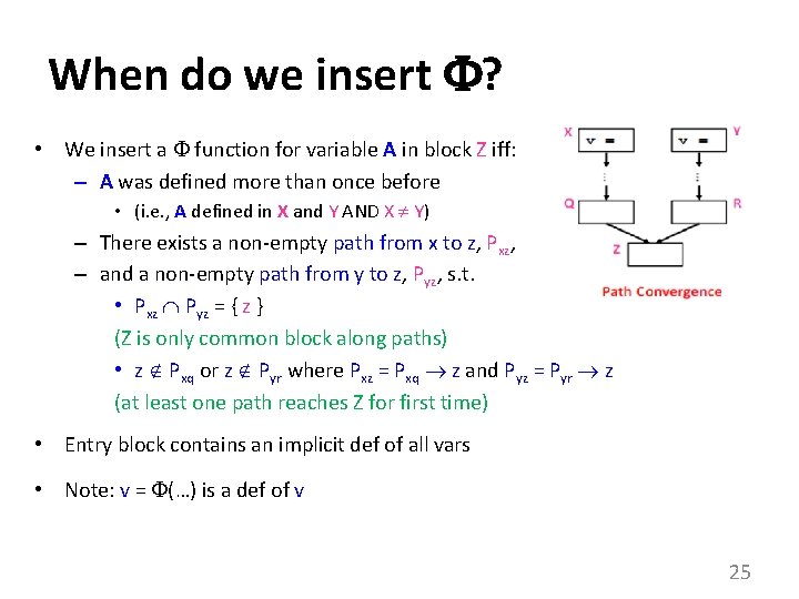
When do we insert ? • We insert a function for variable A in block Z iff: – A was defined more than once before • (i. e. , A defined in X and Y AND X Y) – There exists a non-empty path from x to z, Pxz, – and a non-empty path from y to z, Pyz, s. t. • Pxz Pyz = { z } (Z is only common block along paths) • z Pxq or z Pyr where Pxz = Pxq z and Pyz = Pyr z (at least one path reaches Z for first time) • Entry block contains an implicit def of all vars • Note: v = (…) is a def of v 25

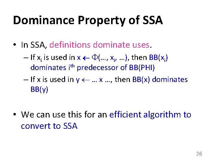
Dominance Property of SSA • In SSA, definitions dominate uses. – If xi is used in x (…, xi, …), then BB(xi) dominates ith predecessor of BB(PHI) – If x is used in y … x …, then BB(x) dominates BB(y) • We can use this for an efficient algorithm to convert to SSA 26

Dominance 1 1 2 3 5 6 7 8 4 2 9 11 10 12 3 4 5 6 7 9 8 10 12 11 If there is a def of a in block 5, which nodes need a ()? 13 CFG D-Tree x strictly dominates w (x sdom w) iff x dom w AND x w 27 13

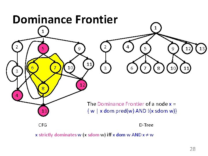
Dominance Frontier 1 1 2 3 5 6 7 8 2 9 11 10 3 4 5 6 7 9 8 10 12 11 12 4 13 CFG The Dominance Frontier of a node x = { w | x dom pred(w) AND !(x sdom w)} D-Tree x strictly dominates w (x sdom w) iff x dom w AND x w 28 13

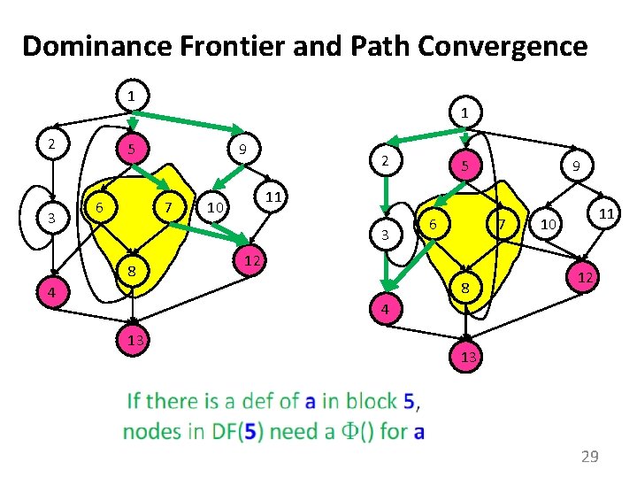
Dominance Frontier and Path Convergence 1 2 3 1 5 6 9 7 2 4 9 11 10 3 8 5 6 7 12 8 11 10 12 4 13 13 29

Using Dominance Frontier to Compute SSA • place all () • Rename all variables 30

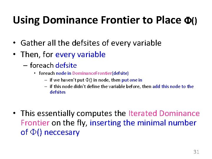
Using Dominance Frontier to Place () • Gather all the defsites of every variable • Then, for every variable – foreach defsite • foreach node in Dominance. Frontier(defsite) – if we haven’t put () in node, then put one in – if this node didn’t define the variable before, then add this node to the defsites • This essentially computes the Iterated Dominance Frontier on the fly, inserting the minimal number of () neccesary 31

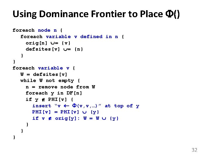
Using Dominance Frontier to Place () foreach node n { foreach variable v defined in n { orig[n] = {v} defsites[v] = {n} } } foreach variable v { W = defsites[v] while W not empty { n = remove node from W foreach y in DF[n] if y PHI[v] { insert “v (v, v, …)” at top of y PHI[v] = PHI[v] {y} if v orig[y]: W = W {y} } 32

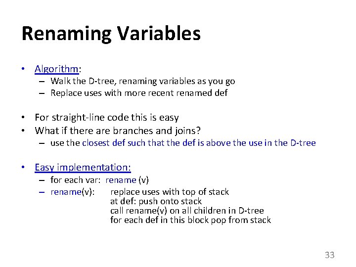
Renaming Variables • Algorithm: – Walk the D-tree, renaming variables as you go – Replace uses with more recent renamed def • For straight-line code this is easy • What if there are branches and joins? – use the closest def such that the def is above the use in the D-tree • Easy implementation: – for each var: rename (v) – rename(v): replace uses with top of stack at def: push onto stack call rename(v) on all children in D-tree for each def in this block pop from stack 33

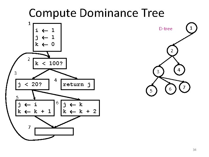
Compute Dominance Tree 1 2 2 k < 100? 4 3 3 j < 20? 4 1 D-tree i 1 j 1 k 0 return j 5 6 7 5 6 j k j i k k + 1 k k + 2 7 34

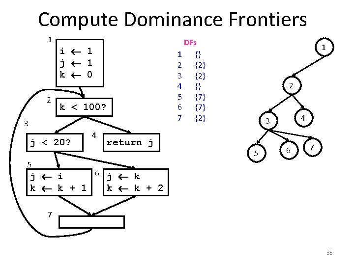
Compute Dominance Frontiers 1 2 DFs 1 {} 2 {2} 3 {2} 4 {} 5 {7} 6 {7} 7 {2} i 1 j 1 k 0 k < 100? 3 j < 20? 4 return j 1 2 4 3 5 6 7 5 6 j k j i k k + 1 k k + 2 7 35

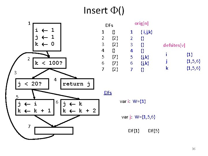
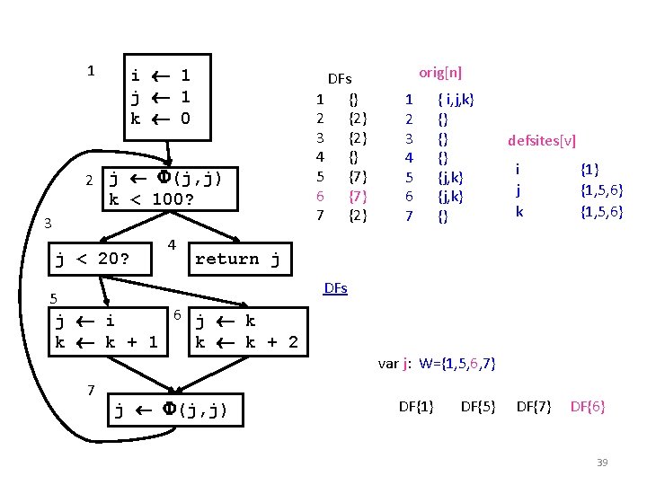
Insert () 1 2 DFs 1 {} 2 {2} 3 {2} 4 {} 5 {7} 6 {7} 7 {2} i 1 j 1 k 0 k < 100? 3 j < 20? 4 orig[n] 1 2 3 4 5 6 7 { i, j, k} {} {j, k} {} defsites[v] i j k {1} {1, 5, 6} return j DFs 5 6 j k j i k k + 1 k k + 2 7 var i: W={1} DF{1} var j: W={1, 5, 6} DF{1} DF{5} 36

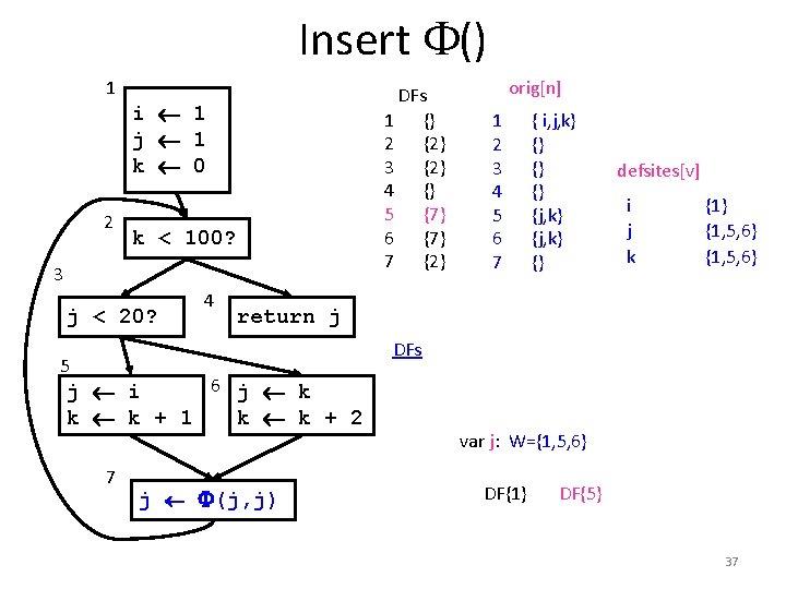
Insert () 1 2 DFs 1 {} 2 {2} 3 {2} 4 {} 5 {7} 6 {7} 7 {2} i 1 j 1 k 0 k < 100? 3 j < 20? 4 orig[n] 1 2 3 4 5 6 7 { i, j, k} {} {j, k} {} defsites[v] i j k {1} {1, 5, 6} return j DFs 5 6 j k j i k k + 1 k k + 2 7 j (j, j) var j: W={1, 5, 6} DF{1} DF{5} 37

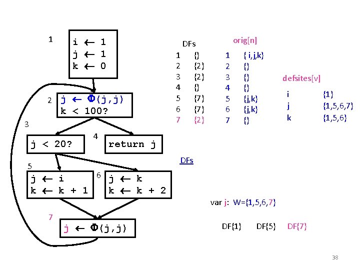
1 i 1 j 1 k 0 2 j (j, j) k < 100? 3 j < 20? 4 DFs 1 {} 2 {2} 3 {2} 4 {} 5 {7} 6 {7} 7 {2} orig[n] 1 2 3 4 5 6 7 { i, j, k} {} {j, k} {} defsites[v] i j k {1} {1, 5, 6, 7} {1, 5, 6} return j DFs 5 6 j k j i k k + 1 k k + 2 var j: W={1, 5, 6, 7} 7 j (j, j) DF{1} DF{5} DF{7} 38

1 i 1 j 1 k 0 2 j (j, j) k < 100? 3 j < 20? 4 DFs 1 {} 2 {2} 3 {2} 4 {} 5 {7} 6 {7} 7 {2} orig[n] 1 2 3 4 5 6 7 { i, j, k} {} {j, k} {} defsites[v] i j k {1} {1, 5, 6} return j DFs 5 6 j k j i k k + 1 k k + 2 var j: W={1, 5, 6, 7} 7 j (j, j) DF{1} DF{5} DF{7} DF{6} 39

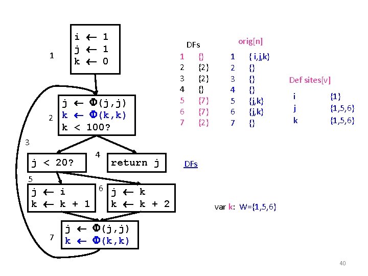
1 i 1 j 1 k 0 j (j, j) 2 k (k, k) k < 100? DFs 1 {} 2 {2} 3 {2} 4 {} 5 {7} 6 {7} 7 {2} orig[n] 1 2 3 4 5 6 7 { i, j, k} {} {j, k} {} Def sites[v] i j k {1} {1, 5, 6} 3 j < 20? 4 return j DFs 5 6 j k j i k k + 1 k k + 2 7 var k: W={1, 5, 6} j (j, j) k (k, k) 40

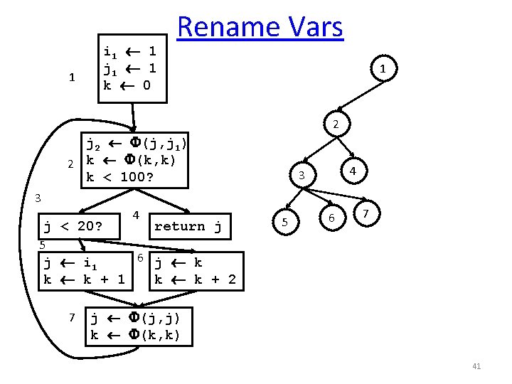
1 i 1 1 j 1 1 k 0 Rename Vars 1 2 j 2 (j, j 1) 2 k (k, k) k < 100? 4 3 3 j < 20? 4 return j 5 6 7 5 6 j k j i 1 k k + 2 7 j (j, j) k (k, k) 41

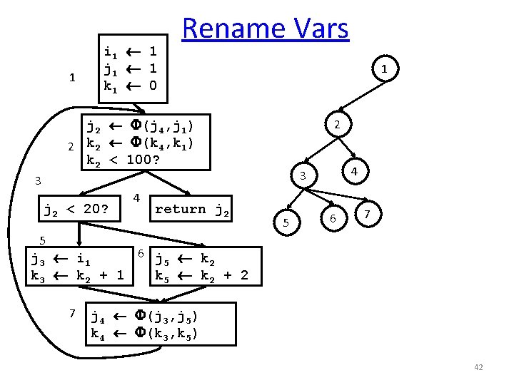
1 i 1 1 j 1 1 k 1 0 Rename Vars 1 j 2 (j 4, j 1) 2 k 2 (k 4, k 1) k 2 < 100? 2 j 2 < 20? 4 return j 2 4 3 3 5 6 7 5 6 j k j 3 i 1 5 2 k 3 k 2 + 1 k 5 k 2 + 2 7 j 4 (j 3, j 5) k 4 (k 3, k 5) 42

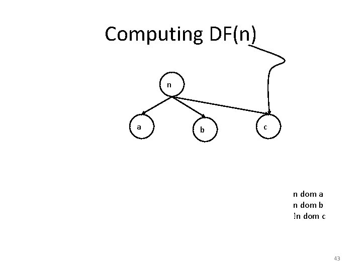
Computing DF(n) n a b c n dom a n dom b !n dom c 43

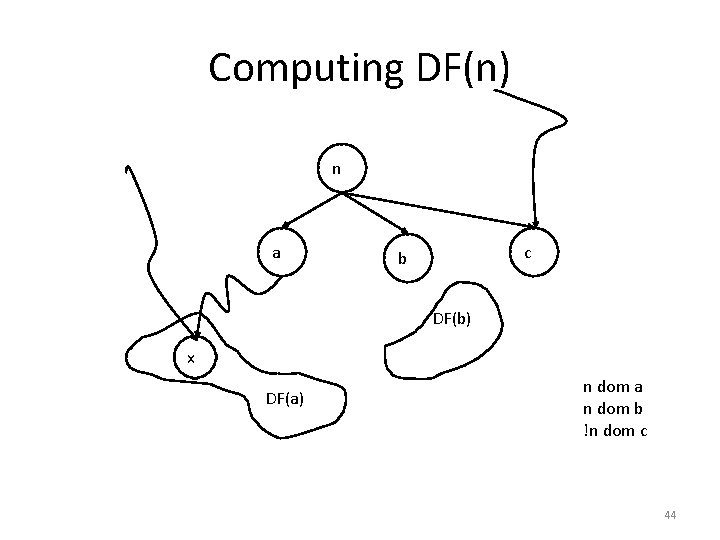
Computing DF(n) n a c b DF(b) x DF(a) n dom a n dom b !n dom c 44

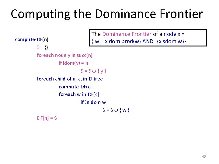
Computing the Dominance Frontier The Dominance Frontier of a node x = { w | x dom pred(w) AND !(x sdom w)} compute-DF(n) S = {} foreach node y in succ[n] if idom(y) n S=S {y} foreach child of n, c, in D-tree compute-DF(c) foreach w in DF[c] if !n dom w S=S {w} DF[n] = S 45

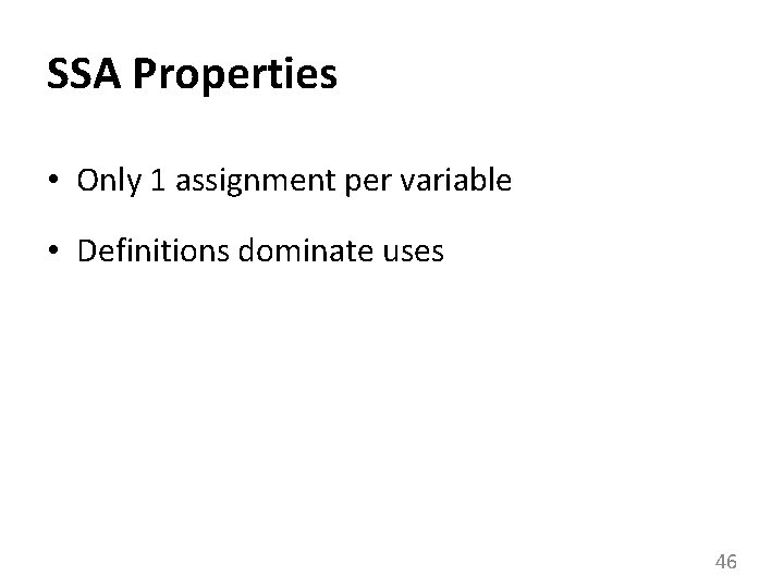
SSA Properties • Only 1 assignment per variable • Definitions dominate uses 46

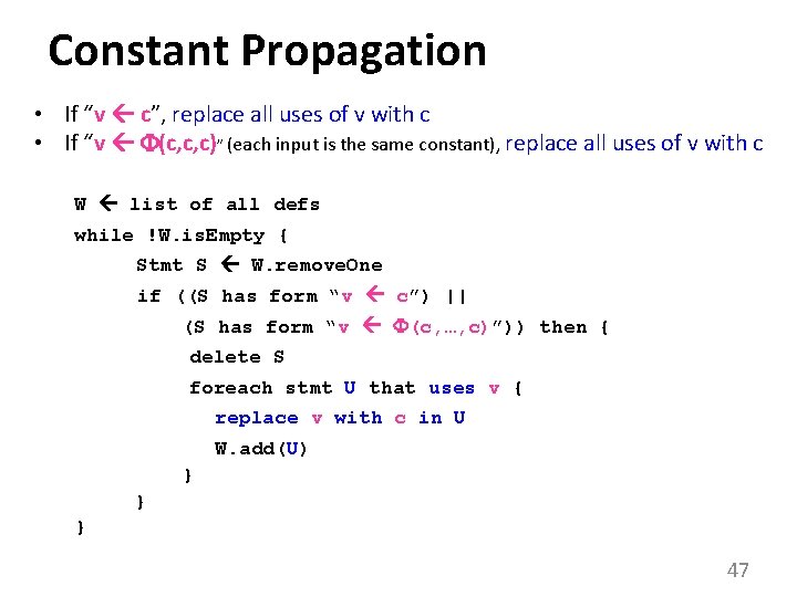
Constant Propagation • If “v c”, replace all uses of v with c • If “v (c, c, c)” (each input is the same constant), replace all uses of v with c W list of all defs while !W. is. Empty { Stmt S W. remove. One if ((S has form “v c”) || (S has form “v (c, …, c)”)) then { delete S foreach stmt U that uses v { replace v with c in U W. add(U) } } } 47

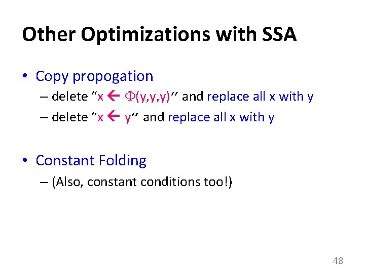
Other Optimizations with SSA • Copy propogation – delete “x (y, y, y)” and replace all x with y – delete “x y” and replace all x with y • Constant Folding – (Also, constant conditions too!) 48

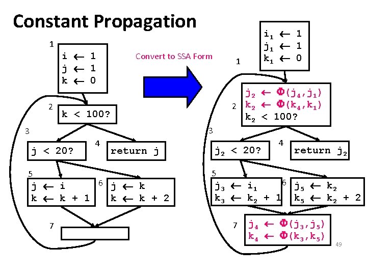
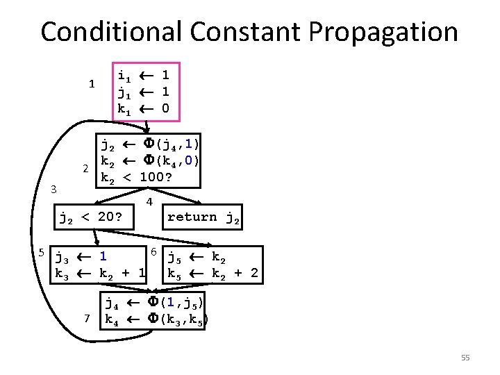
Constant Propagation 1 2 i 1 j 1 k 0 Convert to SSA Form i 1 1 j 1 1 k 1 0 1 j 2 (j 4, j 1) 2 k 2 (k 4, k 1) k 2 < 100? k < 100? 3 3 j < 20? 5 4 return j 6 j k j i k k + 1 k k + 2 7 j 2 < 20? 4 return j 2 5 6 j k j 3 i 1 5 2 k 3 k 2 + 1 k 5 k 2 + 2 7 j 4 (j 3, j 5) k 4 (k 3, k 5) 49

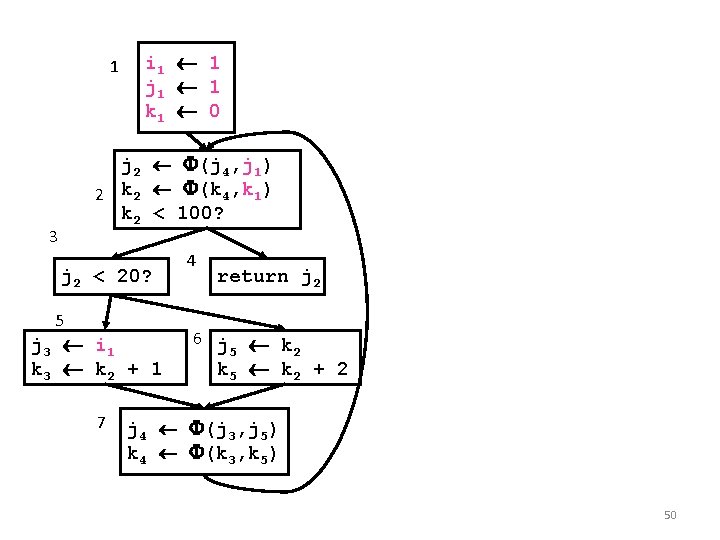
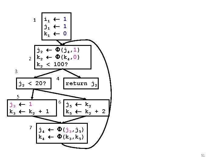
1 i 1 1 j 1 1 k 1 0 j 2 (j 4, j 1) 2 k 2 (k 4, k 1) k 2 < 100? 3 j 2 < 20? 5 j 3 i 1 k 3 k 2 + 1 7 4 return j 2 6 j k 5 2 k 5 k 2 + 2 j 4 (j 3, j 5) k 4 (k 3, k 5) 50

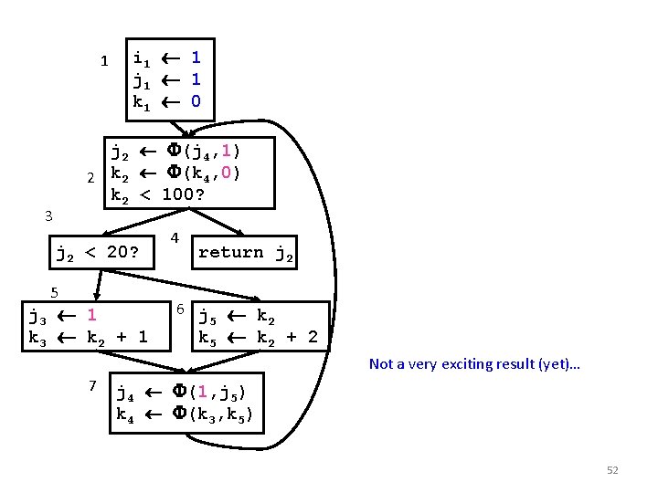
1 i 1 1 j 1 1 k 1 0 j 2 (j 4, 1) 2 k 2 (k 4, 0) k 2 < 100? 3 j 2 < 20? 5 j 3 1 k 3 k 2 + 1 7 4 return j 2 6 j k 5 2 k 5 k 2 + 2 j 4 (j 3, j 5) k 4 (k 3, k 5) 51

1 i 1 1 j 1 1 k 1 0 j 2 (j 4, 1) 2 k 2 (k 4, 0) k 2 < 100? 3 j 2 < 20? 5 j 3 1 k 3 k 2 + 1 4 return j 2 6 j k 5 2 k 5 k 2 + 2 Not a very exciting result (yet)… 7 j 4 (1, j 5) k 4 (k 3, k 5) 52

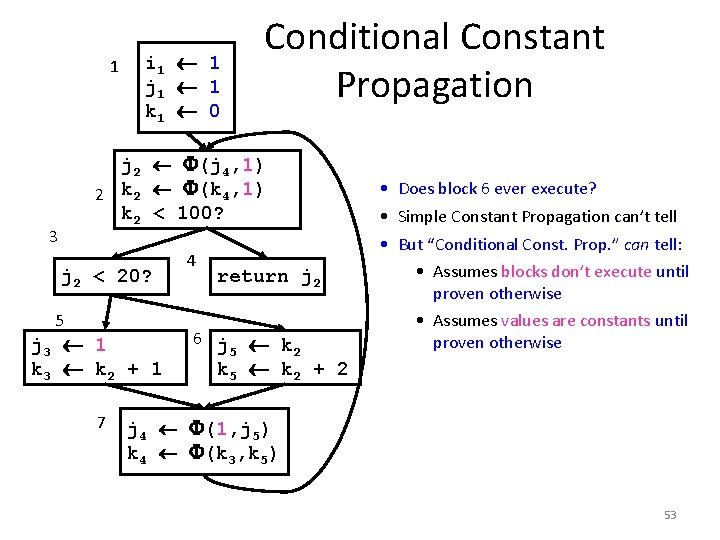
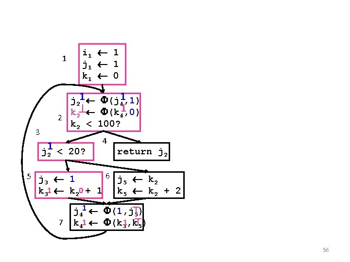
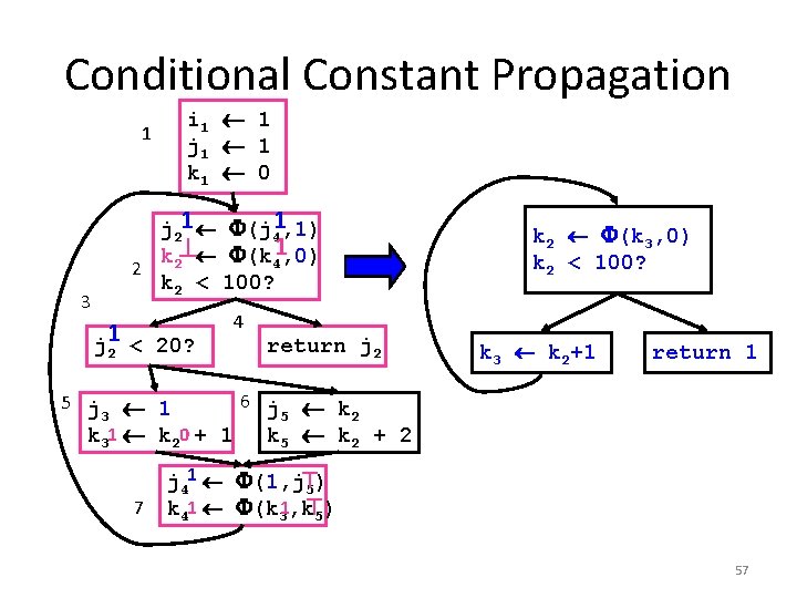
1 i 1 1 j 1 1 k 1 0 Conditional Constant Propagation j 2 (j 4, 1) 2 k 2 (k 4, 1) k 2 < 100? 3 j 2 < 20? 5 j 3 1 k 3 k 2 + 1 7 4 return j 2 6 j k 5 2 • Does block 6 ever execute? • Simple Constant Propagation can’t tell • But “Conditional Const. Prop. ” can tell: • Assumes blocks don’t execute until proven otherwise • Assumes values are constants until proven otherwise k 5 k 2 + 2 j 4 (1, j 5) k 4 (k 3, k 5) 53

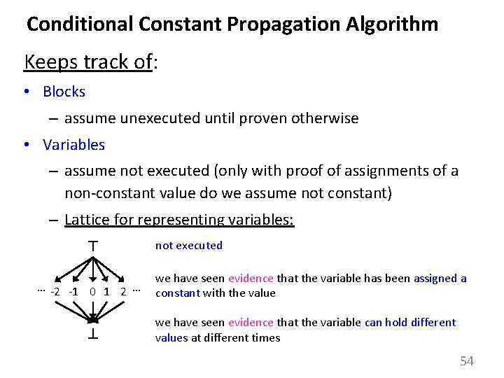
Conditional Constant Propagation Algorithm Keeps track of: • Blocks – assume unexecuted until proven otherwise • Variables – assume not executed (only with proof of assignments of a non-constant value do we assume not constant) – Lattice for representing variables: … -2 -1 0 1 2 … not executed we have seen evidence that the variable has been assigned a constant with the value we have seen evidence that the variable can hold different values at different times 54

Conditional Constant Propagation i 1 1 j 1 1 k 1 0 1 3 j 2 (j 4, 1) k 2 (k 4, 0) 2 k 2 < 100? j 2 < 20? 5 j 1 3 k 3 k 2 + 1 7 4 return j 2 6 j k 5 2 k 5 k 2 + 2 j 4 (1, j 5) k 4 (k 3, k 5) 55

1 3 i 1 1 j 1 1 k 1 0 j 21 (j 41, 1) k 2 (k 41, 0) 2 k 2 < 100? j 1 2 < 20? 4 return j 2 6 j k 5 j 1 3 5 2 k 31 k 20 + 1 k 5 k 2 + 2 7 j 41 (1, j 5) k 41 (k 31, k 5) 56

Conditional Constant Propagation 1 3 i 1 1 j 1 1 k 1 0 j 21 (j 41, 1) k 2 (k 41, 0) 2 k 2 < 100? j 1 2 < 20? 4 return j 2 k 2 (k 3, 0) k 2 < 100? k 3 k 2+1 return 1 6 j k 5 j 1 3 5 2 k 31 k 20 + 1 k 5 k 2 + 2 7 j 41 (1, j 5) k 41 (k 31, k 5) 57

CSC D 70: Compiler Optimization Static Single Assignment (SSA) Prof. Gennady Pekhimenko University of Toronto Winter 2020 The content of this lecture is adapted from the lectures of Todd Mowry and Phillip Gibbons

Backup Slides 59