CS 1704 Introduction to Data Structures and Software

CS 1704 Introduction to Data Structures and Software Engineering

Sorting Terms & Definitions Internal sorts holds all data in RAM n External sorts use Files n Ascending Order: n – Low to High n Descending Order: – High to Low n Stable Sort – Maintains the relative order of equal elements, in situ. – Desirable if list is almost sorted or if items with equal values are to also be ordered on a secondary field.

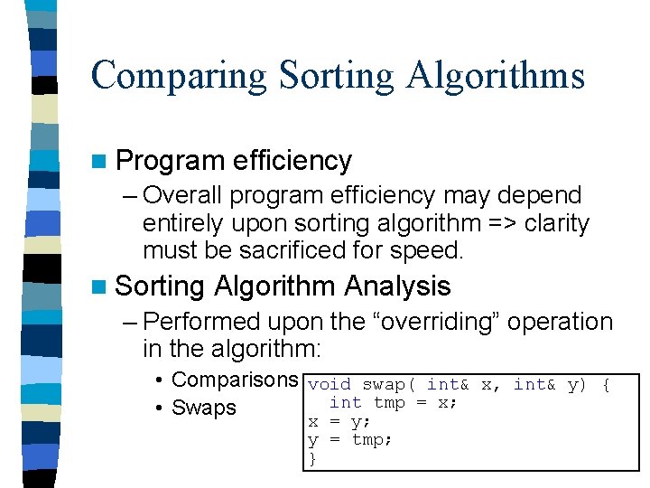
Comparing Sorting Algorithms n Program efficiency – Overall program efficiency may depend entirely upon sorting algorithm => clarity must be sacrificed for speed. n Sorting Algorithm Analysis – Performed upon the “overriding” operation in the algorithm: • Comparisons void swap( int& x, int& y) { int tmp = x; • Swaps x = y; y = tmp; }

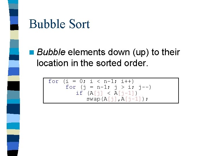
Bubble Sort n Bubble elements down (up) to their location in the sorted order. for (i = 0; i < n-1; i++) for (j = n-1; j > i; j--) if (A[j] < A[j-1]) swap(A[j], A[j-1]);

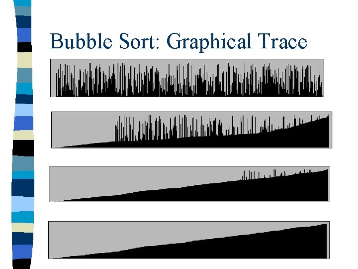
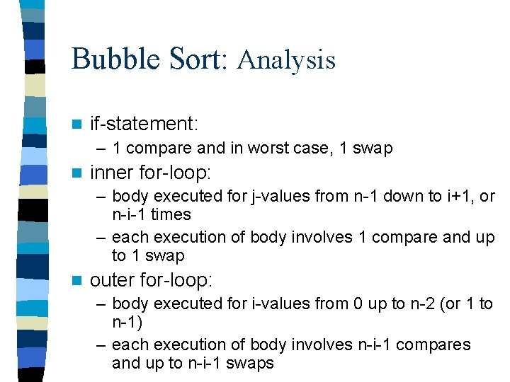
Bubble Sort: Graphical Trace

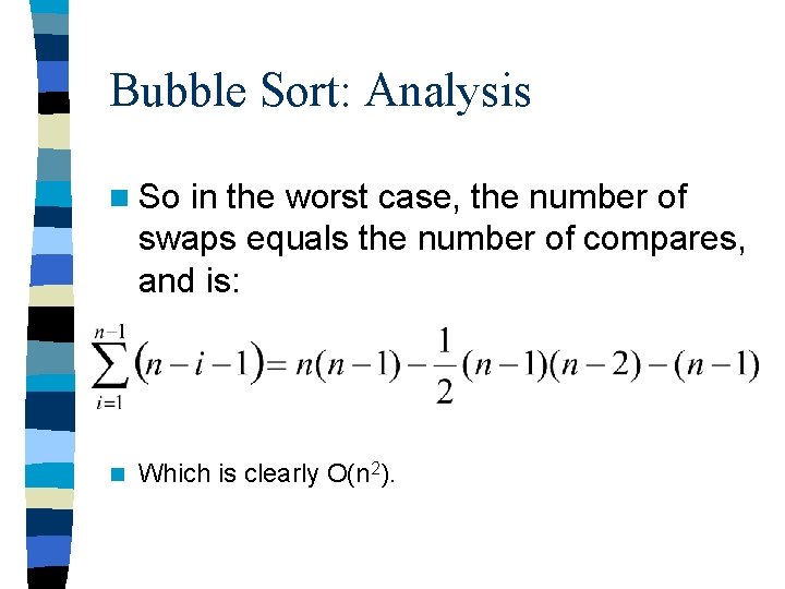
Bubble Sort: Analysis n if-statement: – 1 compare and in worst case, 1 swap n inner for-loop: – body executed for j-values from n-1 down to i+1, or n-i-1 times – each execution of body involves 1 compare and up to 1 swap n outer for-loop: – body executed for i-values from 0 up to n-2 (or 1 to n-1) – each execution of body involves n-i-1 compares and up to n-i-1 swaps

Bubble Sort: Analysis n So in the worst case, the number of swaps equals the number of compares, and is: n Which is clearly O(n 2).

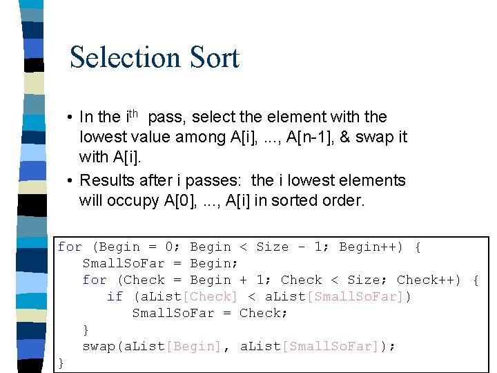
Selection Sort • In the ith pass, select the element with the lowest value among A[i], . . . , A[n-1], & swap it with A[i]. • Results after i passes: the i lowest elements will occupy A[0], . . . , A[i] in sorted order. for (Begin = 0; Begin < Size - 1; Begin++) { Small. So. Far = Begin; for (Check = Begin + 1; Check < Size; Check++) { if (a. List[Check] < a. List[Small. So. Far]) Small. So. Far = Check; } swap(a. List[Begin], a. List[Small. So. Far]); }

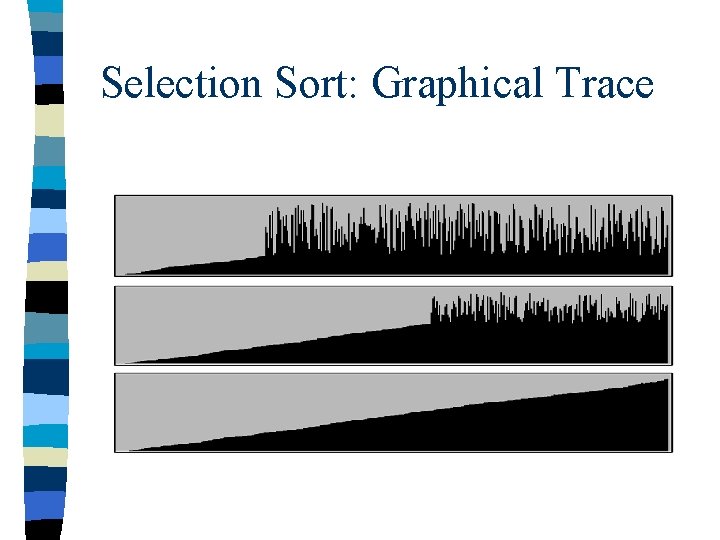
Selection Sort: Graphical Trace

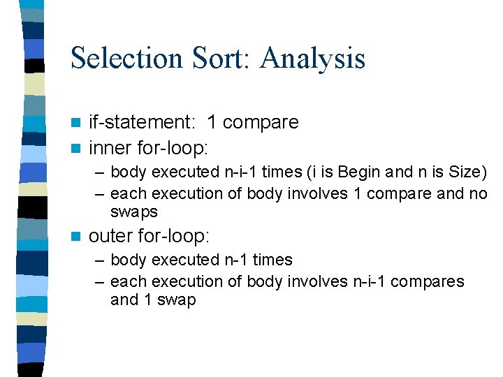
Selection Sort: Analysis if-statement: 1 compare n inner for-loop: n – body executed n-i-1 times (i is Begin and n is Size) – each execution of body involves 1 compare and no swaps n outer for-loop: – body executed n-1 times – each execution of body involves n-i-1 compares and 1 swap

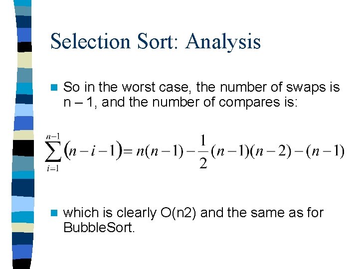
Selection Sort: Analysis n So in the worst case, the number of swaps is n – 1, and the number of compares is: n which is clearly O(n 2) and the same as for Bubble. Sort.

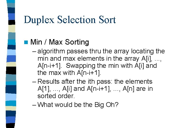
Duplex Selection Sort n Min / Max Sorting – algorithm passes thru the array locating the min and max elements in the array A[i], . . . , A[n-i+1]. Swapping the min with A[i] and the max with A[n-i+1]. – Results after the ith pass: the elements A[1], . . . , A[i] and A[n-i+1], . . . , A[n] are in sorted order. – What would be the Big Oh?

Duplex Selection Sort Analysis n Without going through the figures, – Duplex Selection Sort is another O(N 2) sort algorithm. – But, the coefficient IS better than for Bubble. Sort!

Sorting Thoughts n Comparison-Based Sorting – Algorithms which compare element values to each other – What is the minimum number of comparisons, required to sort N elements using a comparison-based sort? n Is a Queue a type of sorting?

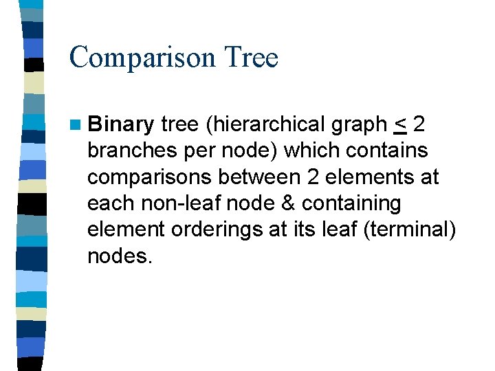
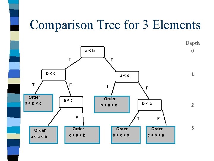
Comparison Tree n Binary tree (hierarchical graph < 2 branches per node) which contains comparisons between 2 elements at each non-leaf node & containing element orderings at its leaf (terminal) nodes.

Comparison Tree for 3 Elements Depth 0 a<b T F b<c T F Order a<b<c a<c T Order a<c<b 1 a<c T F Order b<a<c b<c F Order c<a<b T Order b<c<a 2 F Order c<b<a 3

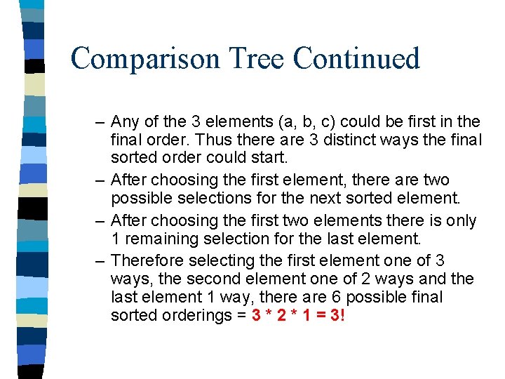
Comparison Tree Continued – Any of the 3 elements (a, b, c) could be first in the final order. Thus there are 3 distinct ways the final sorted order could start. – After choosing the first element, there are two possible selections for the next sorted element. – After choosing the first two elements there is only 1 remaining selection for the last element. – Therefore selecting the first element one of 3 ways, the second element one of 2 ways and the last element 1 way, there are 6 possible final sorted orderings = 3 * 2 * 1 = 3!

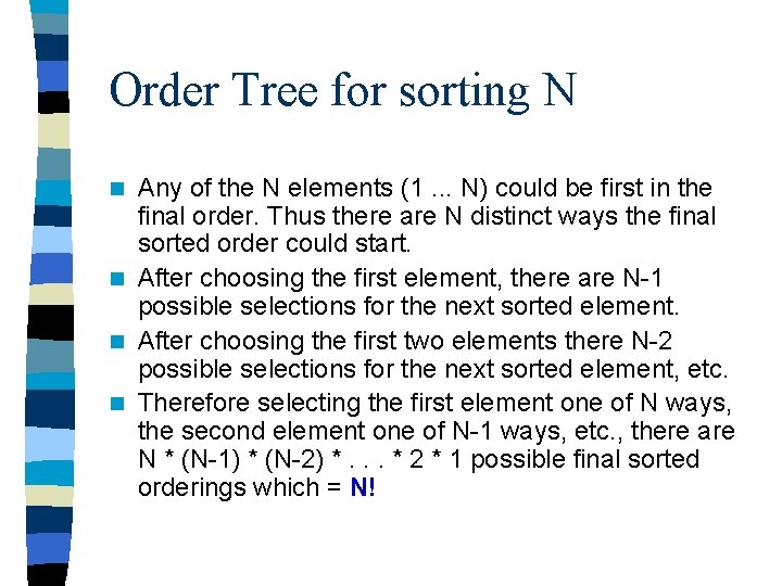
Order Tree for sorting N Any of the N elements (1. . . N) could be first in the final order. Thus there are N distinct ways the final sorted order could start. n After choosing the first element, there are N-1 possible selections for the next sorted element. n After choosing the first two elements there N-2 possible selections for the next sorted element, etc. n Therefore selecting the first element one of N ways, the second element one of N-1 ways, etc. , there are N * (N-1) * (N-2) *. . . * 2 * 1 possible final sorted orderings which = N! n

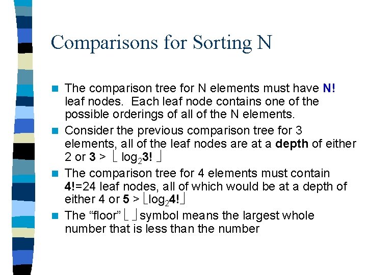
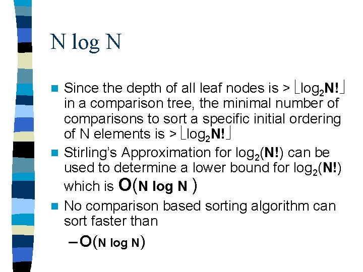
Comparisons for Sorting N The comparison tree for N elements must have N! leaf nodes. Each leaf node contains one of the possible orderings of all of the N elements. n Consider the previous comparison tree for 3 elements, all of the leaf nodes are at a depth of either 2 or 3 > log 23! n The comparison tree for 4 elements must contain 4!=24 leaf nodes, all of which would be at a depth of either 4 or 5 > log 24! n The “floor” symbol means the largest whole number that is less than the number n

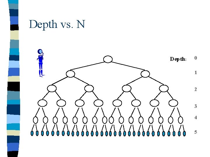
Depth vs. N Depth: 0 1 2 3 4 5

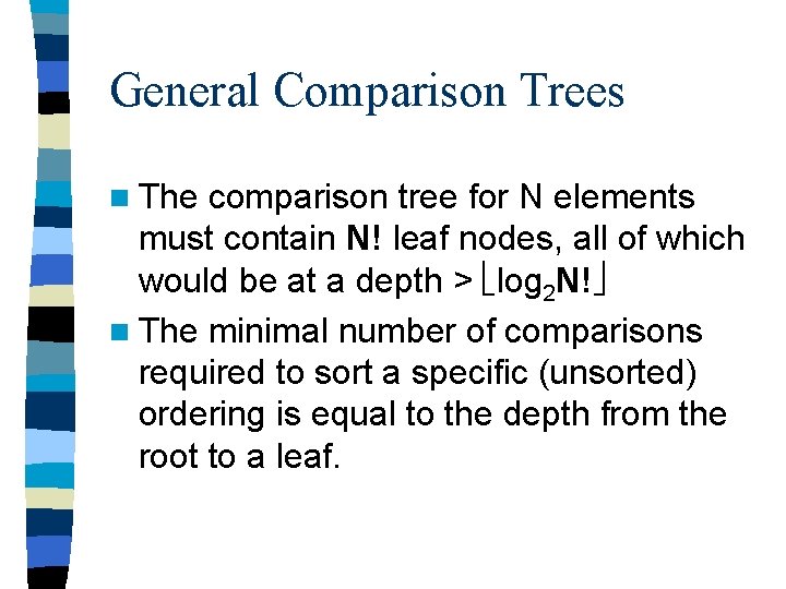
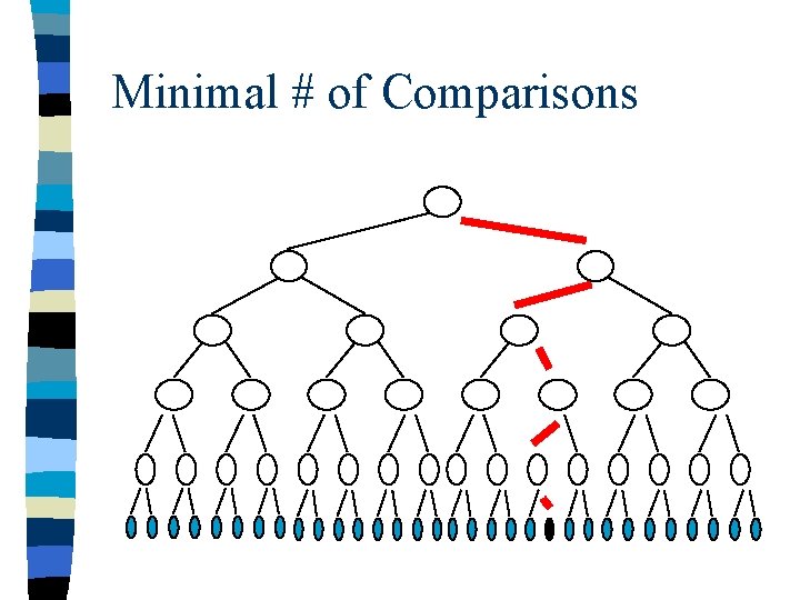
General Comparison Trees n The comparison tree for N elements must contain N! leaf nodes, all of which would be at a depth > log 2 N! n The minimal number of comparisons required to sort a specific (unsorted) ordering is equal to the depth from the root to a leaf.

Minimal # of Comparisons

N log N Since the depth of all leaf nodes is > log 2 N! in a comparison tree, the minimal number of comparisons to sort a specific initial ordering of N elements is > log 2 N! n Stirling’s Approximation for log 2(N!) can be used to determine a lower bound for log 2(N!) which is O(N log N ) n No comparison based sorting algorithm can sort faster than n – O(N log N)

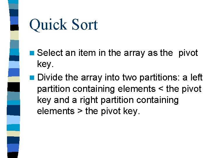
Quick Sort n Select an item in the array as the pivot key. n Divide the array into two partitions: a left partition containing elements < the pivot key and a right partition containing elements > the pivot key.

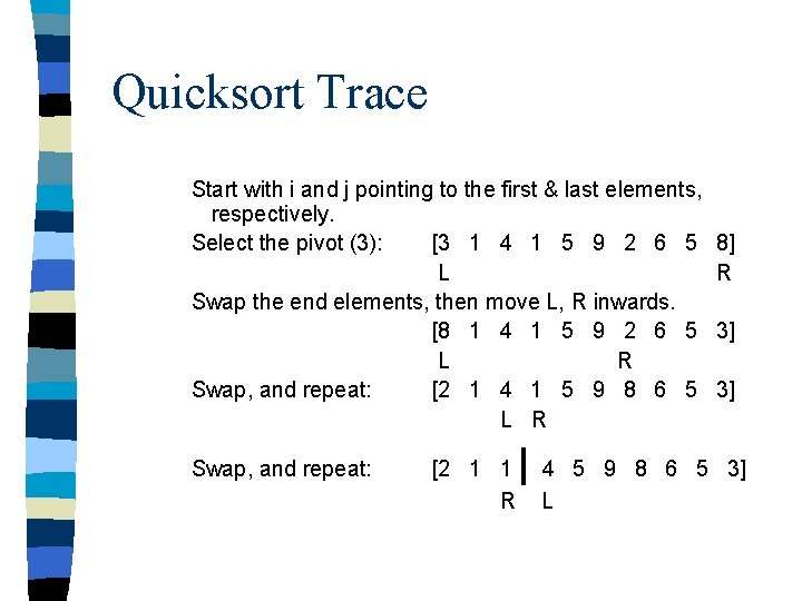
Quicksort Trace Start with i and j pointing to the first & last elements, respectively. Select the pivot (3): [3 1 4 1 5 9 2 6 5 L Swap the end elements, then move L, R inwards. [8 1 4 1 5 9 2 6 5 L R Swap, and repeat: [2 1 4 1 5 9 8 6 5 L R Swap, and repeat: [2 1 1 R | 8] R 3] 3] 4 5 9 8 6 5 3] L

Quicksort int Partition(Item A[], int start, int end, const Item& pivot ){ int L = start, R = end; } do { swap( A[L] , A[R] ); while (A[L] < pivot ) while (!(A[R] < pivot)) } while (R > L); return (L); L++; R--; //< overloaded

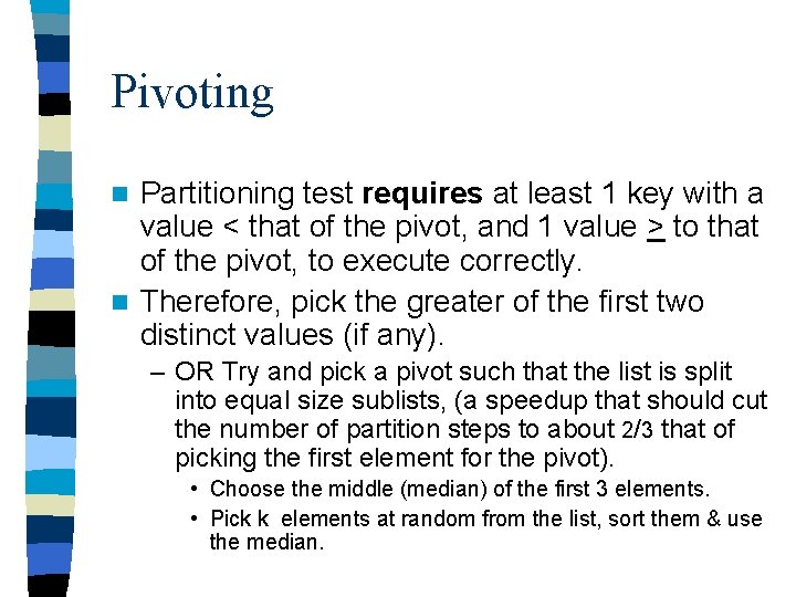
Pivoting Partitioning test requires at least 1 key with a value < that of the pivot, and 1 value > to that of the pivot, to execute correctly. n Therefore, pick the greater of the first two distinct values (if any). n – OR Try and pick a pivot such that the list is split into equal size sublists, (a speedup that should cut the number of partition steps to about 2/3 that of picking the first element for the pivot). • Choose the middle (median) of the first 3 elements. • Pick k elements at random from the list, sort them & use the median.

Find Pivot const int MISSING = -1; int Find. Pivot(const Item A[], int start, int end ) { Item firstkey; //value of first key found int pivot; //pivot index int k; //run right looking for other key } firstkey = A[start]; //return -1 if different keys are not found pivot = MISSING; k = start + 1; //scan for different key while ( (k <= end) && (pivot == MISSING) ) if (firstkey < A[k]) //select key pivot = k; else if (A[k] < firstkey) pivot = start; else k++; return pivot;

Quick Sort Function const int MISSING = -1; void Quick. Sort( Item A[], int start, int end ) { // sort the array from start. . . end Item pivot. Key; int pivot. Index; int k; //index of partition >= pivot } pivot. Index = Find. Pivot( A, start, end ); if (pivot. Index != MISSING) { pivot. Key = A[pivot. Index]; k = Partition( A, start, end, pivot. Key ); Quick. Sort( A, start, k-1 ); Quick. Sort( A, k, end ); }

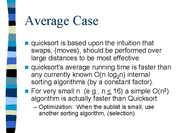
Average Case quicksort is based upon the intuition that swaps, (moves), should be performed over large distances to be most effective. n quicksort's average running time is faster than any currently known O(n log 2 n) internal sorting algorithms (by a constant factor). n For very small n (e. g. , n < 16) a simple O(n 2) algorithm is actually faster than Quicksort. n – Optimization: When the sublist is small, use another sorting algorithm, (selection).

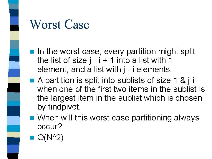
Worst Case In the worst case, every partition might split the list of size j - i + 1 into a list with 1 element, and a list with j - i elements. n A partition is split into sublists of size 1 & j-i when one of the first two items in the sublist is the largest item in the sublist which is chosen by findpivot. n When will this worst case partitioning always occur? n O(N^2) n

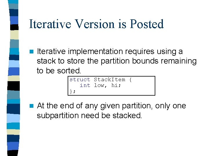
Iterative Version is Posted n Iterative implementation requires using a stack to store the partition bounds remaining to be sorted. struct Stack. Item { int low, hi; }; n At the end of any given partition, only one subpartition need be stacked.

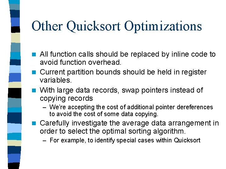
Other Quicksort Optimizations All function calls should be replaced by inline code to avoid function overhead. n Current partition bounds should be held in register variables. n With large data records, swap pointers instead of copying records n – We’re accepting the cost of additional pointer dereferences to avoid the cost of some data copying. n Carefully investigate the average data arrangement in order to select the optimal sorting algorithm. – For example, to identify special cases within Quicksort

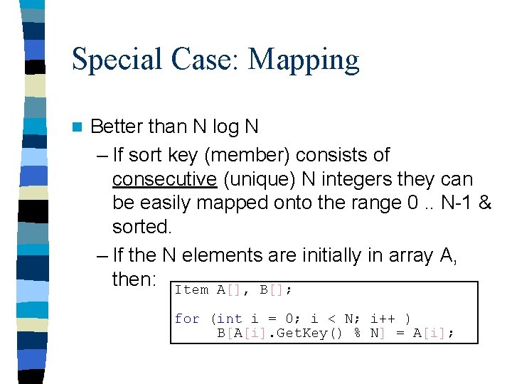
Special Case: Mapping n Better than N log N – If sort key (member) consists of consecutive (unique) N integers they can be easily mapped onto the range 0. . N-1 & sorted. – If the N elements are initially in array A, then: Item A[], B[]; for (int i = 0; i < N; i++ ) B[A[i]. Get. Key() % N] = A[i];

Mapping takes O(n) time. n Requires exactly 1 record with each key value! n Of course, this is a very special circumstance… n Special case of Bin Sorting. (If integers are not consecutive, but within a reasonable range, bit flags can be used to denote empty array slots. ) n

Bin Sorting Assume we need to sort an array of integers in the range 0 -99: n Assume we have an array of 10 linked lists (bins) for storage. n First make a pass through the list of integers, and place each into the bin that matches its 1’s digit. n Then, make a second pass, taking each bin in order, and place each integer into the bin that matches its 2’s digit, etc. n

Bin Sorting n Now if you just read the bins, in order, the elements will appear in ascending order. – Assuming no Bin with > 1 element – Otherwise, use another sort technique to sort bins Each pass takes O(N) work, and the number of passes is just the number of digits in the largest integer in the original list. n That beats Quick. Sort, but only in a somewhat special case. (When each bin has 1 element) n Binsort Implementation posted online. n