COP 3502 Computer Science I Spring 2004 Day

COP 3502: Computer Science I Spring 2004 – Day 10 – Searching and Sorting Instructor : Mark Llewellyn markl@cs. ucf. edu CC 1 211, 823 -2790 http: //www. cs. ucf. edu/courses/cop 3502/spr 04 School of Electrical Engineering and Computer Science University of Central Florida COP 3502: Computer Science I (Day 10) Page 1 © Mark Llewellyn

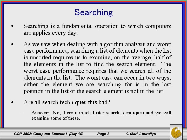
Searching • Searching is a fundamental operation to which computers are applies every day. • As we saw when dealing with algorithm analysis and worst case performance, searching a list of elements when the list is unsorted requires us to examine, on the average, half of the elements in the list to find the search element. The worst case performance requires that we search all of the elements in the list. The worst case can occur in two ways, either the element we are searching for is in the last position in the list or the search element is not in the list. • Are all search techniques this bad? – Answer: No, there a much faster search techniques and we will examine some of these. COP 3502: Computer Science I (Day 10) Page 2 © Mark Llewellyn

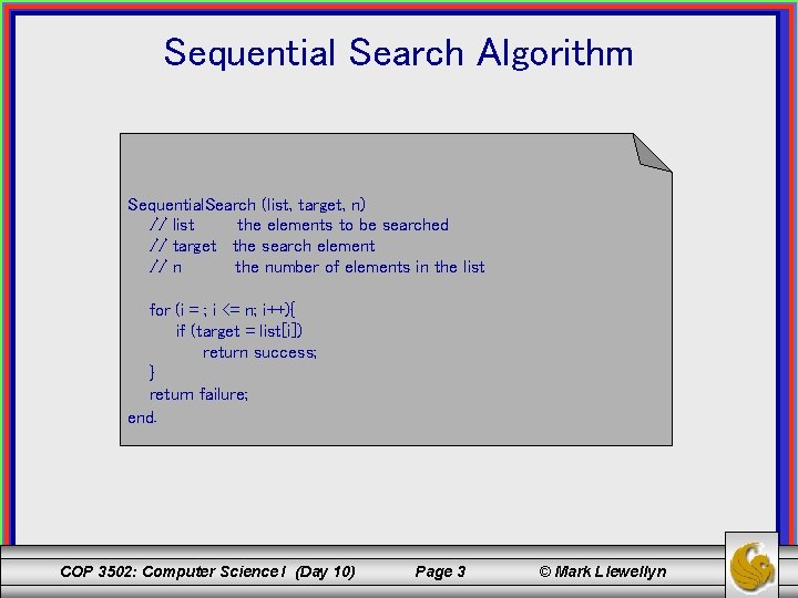
Sequential Search Algorithm Sequential. Search (list, target, n) // list the elements to be searched // target the search element // n the number of elements in the list for (i = ; i <= n; i++){ if (target = list[i]) return success; } return failure; end. COP 3502: Computer Science I (Day 10) Page 3 © Mark Llewellyn

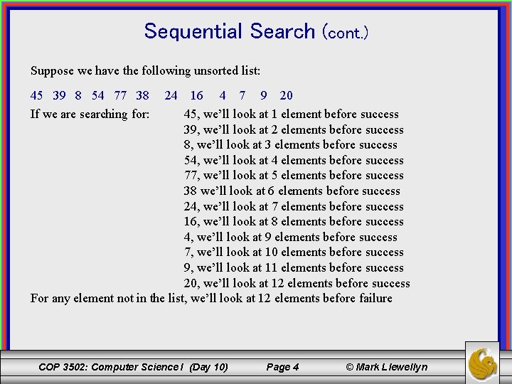
Sequential Search (cont. ) Suppose we have the following unsorted list: 45 39 8 54 77 38 If we are searching for: 24 16 4 7 9 20 45, we’ll look at 1 element before success 39, we’ll look at 2 elements before success 8, we’ll look at 3 elements before success 54, we’ll look at 4 elements before success 77, we’ll look at 5 elements before success 38 we’ll look at 6 elements before success 24, we’ll look at 7 elements before success 16, we’ll look at 8 elements before success 4, we’ll look at 9 elements before success 7, we’ll look at 10 elements before success 9, we’ll look at 11 elements before success 20, we’ll look at 12 elements before success For any element not in the list, we’ll look at 12 elements before failure COP 3502: Computer Science I (Day 10) Page 4 © Mark Llewellyn

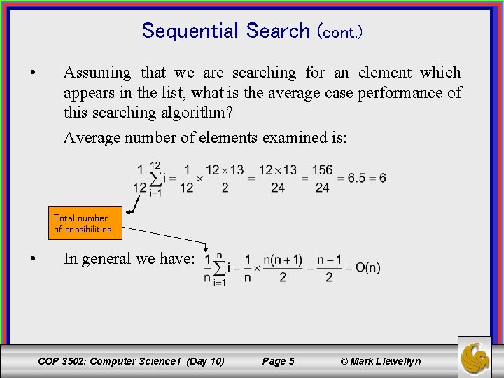
Sequential Search (cont. ) • Assuming that we are searching for an element which appears in the list, what is the average case performance of this searching algorithm? Average number of elements examined is: Total number of possibilities • In general we have: COP 3502: Computer Science I (Day 10) Page 5 © Mark Llewellyn

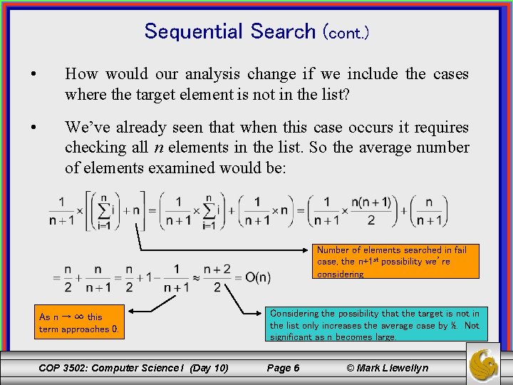
Sequential Search (cont. ) • How would our analysis change if we include the cases where the target element is not in the list? • We’ve already seen that when this case occurs it requires checking all n elements in the list. So the average number of elements examined would be: Number of elements searched in fail case, the n+1 st possibility we’re considering As n → ∞ this term approaches 0. COP 3502: Computer Science I (Day 10) Considering the possibility that the target is not in the list only increases the average case by ½. Not significant as n becomes large. Page 6 © Mark Llewellyn

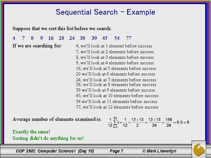
Sequential Search - Example Suppose that we sort this list before we search: 4 7 8 9 16 20 If we are searching for: 24 38 39 45 54 77 4, we’ll look at 1 element before success 7, we’ll look at 2 elements before success 8, we’ll look at 3 elements before success 9, we’ll look at 4 elements before success 16, we’ll look at 5 elements before success 20 we’ll look at 6 elements before success 24, we’ll look at 7 elements before success 38, we’ll look at 8 elements before success 39 we’ll look at 9 elements before success 45, we’ll look at 10 elements before success 54 we’ll look at 11 elements before success 77, we’ll look at 12 elements before success Average number of elements examined is: Exactly the same! Sorting didn’t do anything for us! COP 3502: Computer Science I (Day 10) Page 7 © Mark Llewellyn

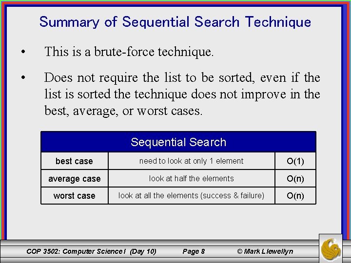
Summary of Sequential Search Technique • This is a brute-force technique. • Does not require the list to be sorted, even if the list is sorted the technique does not improve in the best, average, or worst cases. Sequential Search best case need to look at only 1 element O(1) average case look at half the elements O(n) worst case look at all the elements (success & failure) O(n) COP 3502: Computer Science I (Day 10) Page 8 © Mark Llewellyn

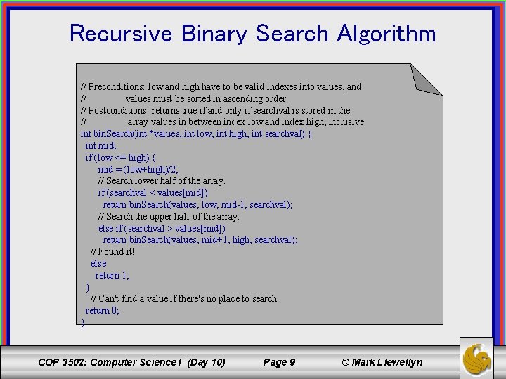
Recursive Binary Search Algorithm // Preconditions: low and high have to be valid indexes into values, and // values must be sorted in ascending order. // Postconditions: returns true if and only if searchval is stored in the // array values in between index low and index high, inclusive. int bin. Search(int *values, int low, int high, int searchval) { int mid; if (low <= high) { mid = (low+high)/2; // Search lower half of the array. if (searchval < values[mid]) return bin. Search(values, low, mid-1, searchval); // Search the upper half of the array. else if (searchval > values[mid]) return bin. Search(values, mid+1, high, searchval); // Found it! else return 1; } // Can't find a value if there's no place to search. return 0; } COP 3502: Computer Science I (Day 10) Page 9 © Mark Llewellyn

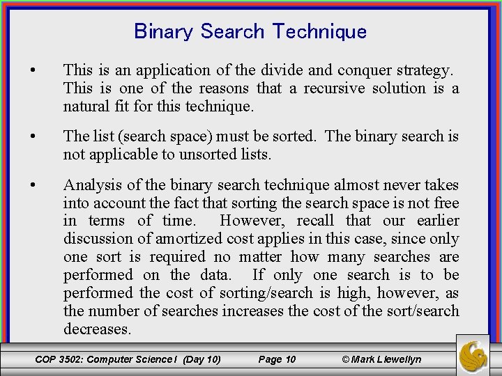
Binary Search Technique • This is an application of the divide and conquer strategy. This is one of the reasons that a recursive solution is a natural fit for this technique. • The list (search space) must be sorted. The binary search is not applicable to unsorted lists. • Analysis of the binary search technique almost never takes into account the fact that sorting the search space is not free in terms of time. However, recall that our earlier discussion of amortized cost applies in this case, since only one sort is required no matter how many searches are performed on the data. If only one search is to be performed the cost of sorting/search is high, however, as the number of searches increases the cost of the sort/search decreases. COP 3502: Computer Science I (Day 10) Page 10 © Mark Llewellyn

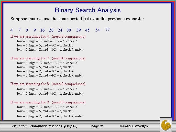
Binary Search Analysis Suppose that we use the same sorted list as in the previous example: 4 7 8 9 16 20 24 38 39 45 54 77 If we are searching for 4: (need 3 comparisons) low = 1, high = 12, mid = 13/2 = 6, check 20 low = 1, high = 5, mid = 6/2 = 3, check 8 low = 1, high = 2, mid = 3/2 = 1, check 4, match If we are searching for 7: (need 4 comparisons) low = 1, high = 12, mid = 13/2 = 6, check 20 low = 1, high = 5, mid = 6/2 = 3, check 8 low = 1, high = 2, mid = 3/2 = 1, check 4 low = 2, high = 2, mid = 4/2 = 2, check 7, match If we are searching for 8: (need 2 comparisons) low = 1, high = 12, mid = 13/2 = 6, check 20 low = 1, high = 5, mid = 6/2 = 3, check 8, match If we are searching for 9: (need 3 comparisons) low = 1, high = 12, mid = 13/2 = 6, check 20 low = 1, high = 5, mid = 6/2 = 3, check 8 low = 1, high = 2, mid = 3/2 = 1, check 4, match COP 3502: Computer Science I (Day 10) Page 11 © Mark Llewellyn

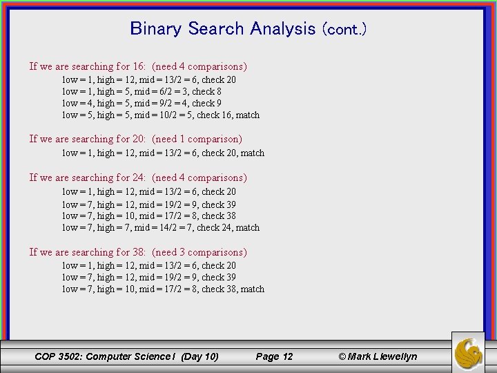
Binary Search Analysis (cont. ) If we are searching for 16: (need 4 comparisons) low = 1, high = 12, mid = 13/2 = 6, check 20 low = 1, high = 5, mid = 6/2 = 3, check 8 low = 4, high = 5, mid = 9/2 = 4, check 9 low = 5, high = 5, mid = 10/2 = 5, check 16, match If we are searching for 20: (need 1 comparison) low = 1, high = 12, mid = 13/2 = 6, check 20, match If we are searching for 24: (need 4 comparisons) low = 1, high = 12, mid = 13/2 = 6, check 20 low = 7, high = 12, mid = 19/2 = 9, check 39 low = 7, high = 10, mid = 17/2 = 8, check 38 low = 7, high = 7, mid = 14/2 = 7, check 24, match If we are searching for 38: (need 3 comparisons) low = 1, high = 12, mid = 13/2 = 6, check 20 low = 7, high = 12, mid = 19/2 = 9, check 39 low = 7, high = 10, mid = 17/2 = 8, check 38, match COP 3502: Computer Science I (Day 10) Page 12 © Mark Llewellyn

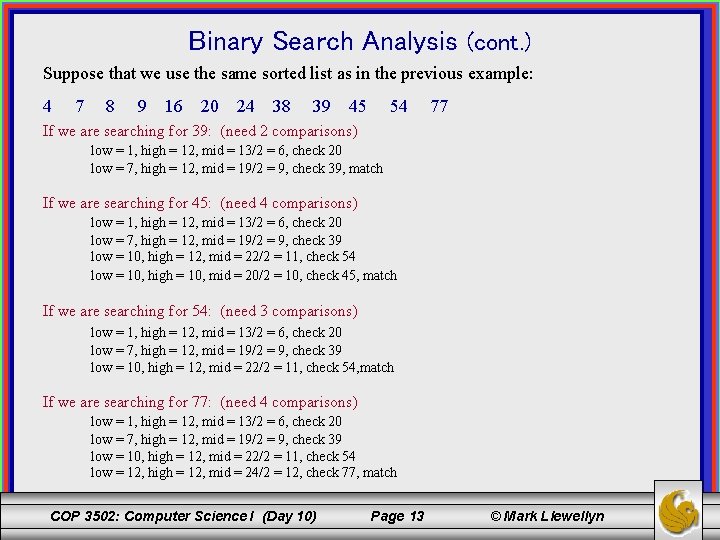
Binary Search Analysis (cont. ) Suppose that we use the same sorted list as in the previous example: 4 7 8 9 16 20 24 38 39 45 54 77 If we are searching for 39: (need 2 comparisons) low = 1, high = 12, mid = 13/2 = 6, check 20 low = 7, high = 12, mid = 19/2 = 9, check 39, match If we are searching for 45: (need 4 comparisons) low = 1, high = 12, mid = 13/2 = 6, check 20 low = 7, high = 12, mid = 19/2 = 9, check 39 low = 10, high = 12, mid = 22/2 = 11, check 54 low = 10, high = 10, mid = 20/2 = 10, check 45, match If we are searching for 54: (need 3 comparisons) low = 1, high = 12, mid = 13/2 = 6, check 20 low = 7, high = 12, mid = 19/2 = 9, check 39 low = 10, high = 12, mid = 22/2 = 11, check 54, match If we are searching for 77: (need 4 comparisons) low = 1, high = 12, mid = 13/2 = 6, check 20 low = 7, high = 12, mid = 19/2 = 9, check 39 low = 10, high = 12, mid = 22/2 = 11, check 54 low = 12, high = 12, mid = 24/2 = 12, check 77, match COP 3502: Computer Science I (Day 10) Page 13 © Mark Llewellyn

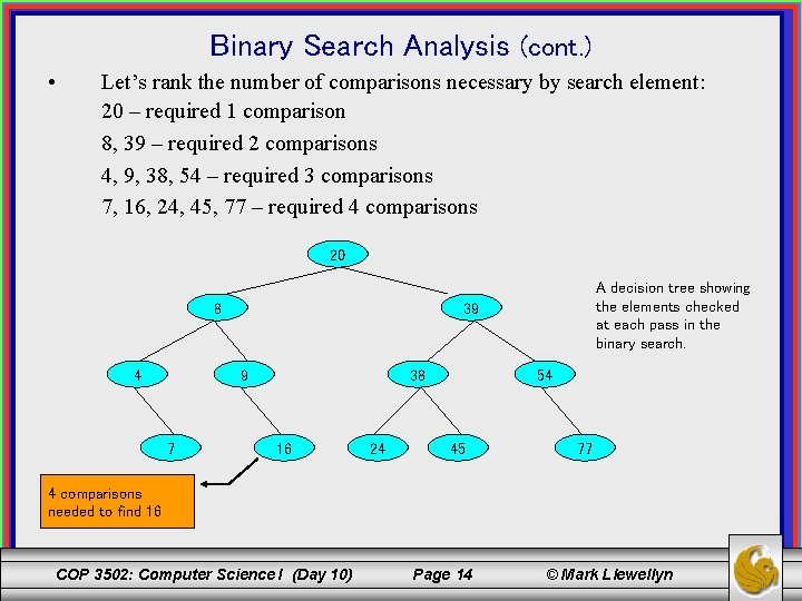
Binary Search Analysis (cont. ) • Let’s rank the number of comparisons necessary by search element: 20 – required 1 comparison 8, 39 – required 2 comparisons 4, 9, 38, 54 – required 3 comparisons 7, 16, 24, 45, 77 – required 4 comparisons 20 8 4 39 9 7 A decision tree showing the elements checked at each pass in the binary search. 38 16 24 54 45 77 4 comparisons needed to find 16 COP 3502: Computer Science I (Day 10) Page 14 © Mark Llewellyn

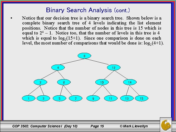
Binary Search Analysis (cont. ) • Notice that our decision tree is a binary search tree. Shown below is a complete binary search tree of 4 levels indicating the list element positions. Notice that the number of nodes in this tree is 15 which is equal to 24 – 1. Notice too, that the number of levels in this tree is 4 which is equal to log 2(15+1). Since one comparison is done on each level, the most number of comparisons that would be done is: log 2(4+1). 8 4 2 1 12 6 3 5 10 7 COP 3502: Computer Science I (Day 10) 9 Page 15 14 11 13 15 © Mark Llewellyn

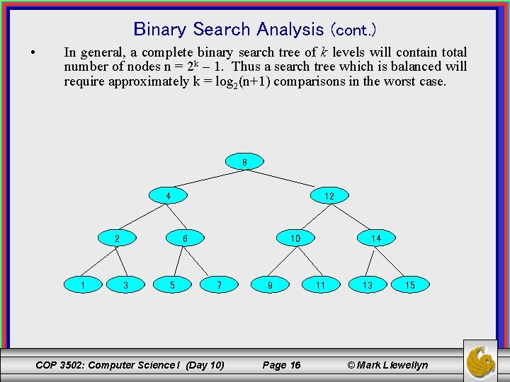
Binary Search Analysis (cont. ) • In general, a complete binary search tree of k levels will contain total number of nodes n = 2 k – 1. Thus a search tree which is balanced will require approximately k = log 2(n+1) comparisons in the worst case. 8 4 2 1 12 6 3 5 10 7 COP 3502: Computer Science I (Day 10) 9 Page 16 14 11 13 15 © Mark Llewellyn

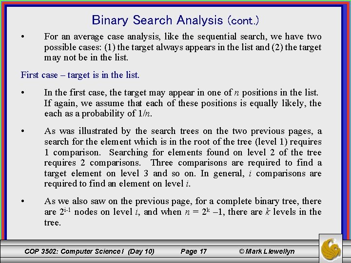
Binary Search Analysis (cont. ) • For an average case analysis, like the sequential search, we have two possible cases: (1) the target always appears in the list and (2) the target may not be in the list. First case – target is in the list. • In the first case, the target may appear in one of n positions in the list. If again, we assume that each of these positions is equally likely, the each as a probability of 1/n. • As was illustrated by the search trees on the two previous pages, a search for the element which is in the root of the tree (level 1) requires 1 comparison. Searching for elements found on level 2 of the tree requires 2 comparisons. Three comparisons are required to find a target element on level 3 and so on. In general, i comparisons are required to find an element on level i. • As we also saw on the previous page, for a complete binary tree, there are 2 i-1 nodes on level i, and when n = 2 k – 1, there are k levels in the tree. COP 3502: Computer Science I (Day 10) Page 17 © Mark Llewellyn

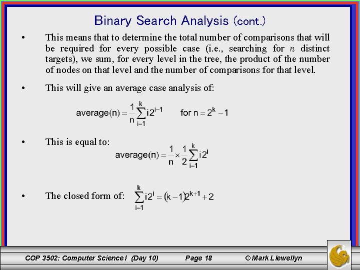
Binary Search Analysis (cont. ) • This means that to determine the total number of comparisons that will be required for every possible case (i. e. , searching for n distinct targets), we sum, for every level in the tree, the product of the number of nodes on that level and the number of comparisons for that level. • This will give an average case analysis of: • This is equal to: • The closed form of: COP 3502: Computer Science I (Day 10) Page 18 © Mark Llewellyn

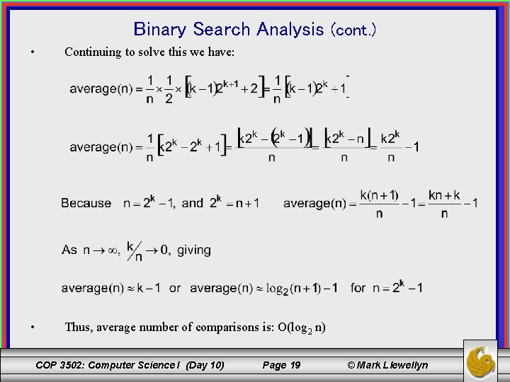
Binary Search Analysis (cont. ) • Continuing to solve this we have: • Thus, average number of comparisons is: O(log 2 n) COP 3502: Computer Science I (Day 10) Page 19 © Mark Llewellyn

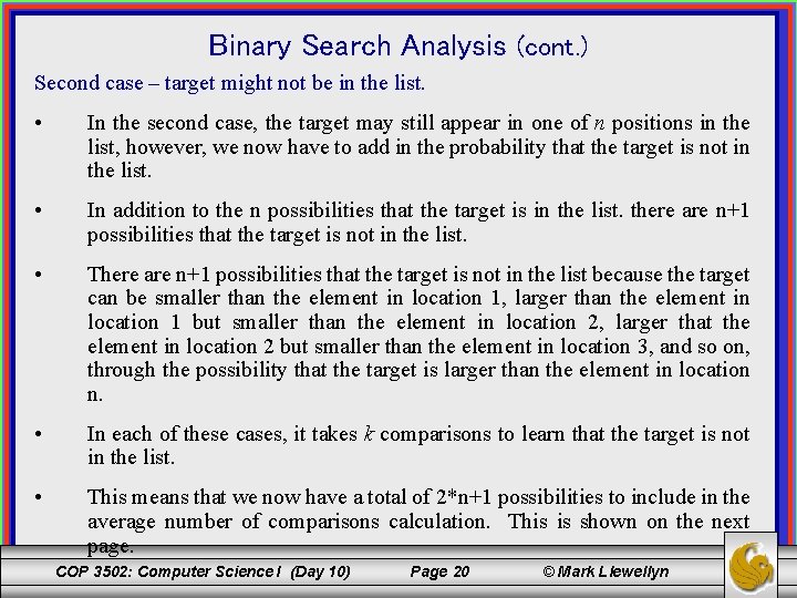
Binary Search Analysis (cont. ) Second case – target might not be in the list. • In the second case, the target may still appear in one of n positions in the list, however, we now have to add in the probability that the target is not in the list. • In addition to the n possibilities that the target is in the list. there are n+1 possibilities that the target is not in the list. • There are n+1 possibilities that the target is not in the list because the target can be smaller than the element in location 1, larger than the element in location 1 but smaller than the element in location 2, larger that the element in location 2 but smaller than the element in location 3, and so on, through the possibility that the target is larger than the element in location n. • In each of these cases, it takes k comparisons to learn that the target is not in the list. • This means that we now have a total of 2*n+1 possibilities to include in the average number of comparisons calculation. This is shown on the next page. COP 3502: Computer Science I (Day 10) Page 20 © Mark Llewellyn

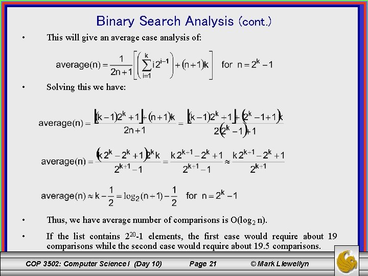
Binary Search Analysis (cont. ) • This will give an average case analysis of: • Solving this we have: • Thus, we have average number of comparisons is O(log 2 n). • If the list contains 220 -1 elements, the first case would require about 19 comparisons while the second case would require about 19. 5 comparisons. COP 3502: Computer Science I (Day 10) Page 21 © Mark Llewellyn

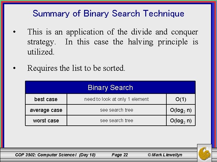
Summary of Binary Search Technique • This is an application of the divide and conquer strategy. In this case the halving principle is utilized. • Requires the list to be sorted. Binary Search best case need to look at only 1 element O(1) average case search tree O(log 2 n) worst case search tree O(log 2 n) COP 3502: Computer Science I (Day 10) Page 22 © Mark Llewellyn

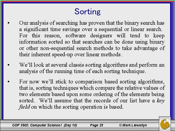
Sorting • Our analysis of searching has proven that the binary search has a significant time savings over a sequential or linear search. For this reason, software designers will tend to keep information sorted so that searches can be done using binary or other non-sequential search methods to take advantage of their inherent speed-up over linear methods. • We’ll look at several classis sorting algorithms and perform an analysis of the running time of each sorting technique. • For now we’ll stick to comparison based sorting algorithms, that is, sorting techniques which compare the relative values of two elements based upon some ordering of the elements being sorted. We’ll assume that the records of our list have a key field on which the sorting operation is based. COP 3502: Computer Science I (Day 10) Page 23 © Mark Llewellyn

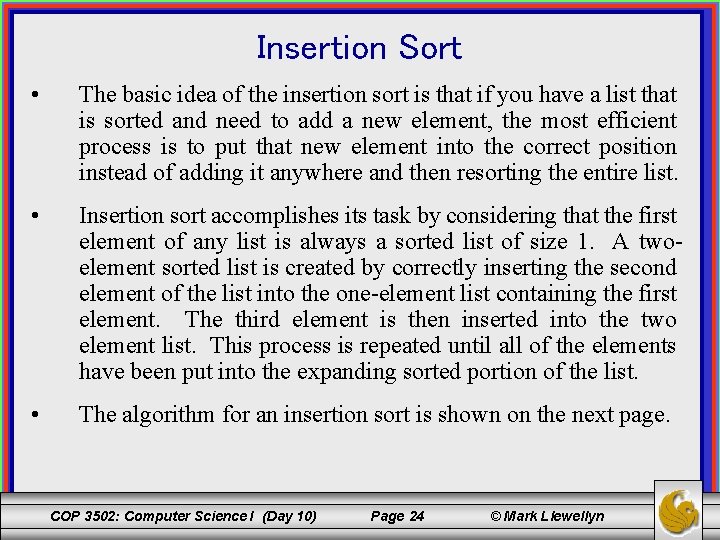
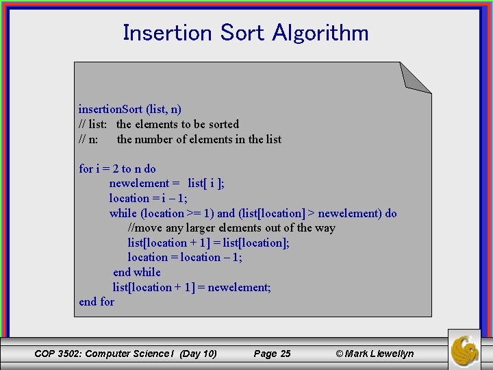
Insertion Sort • The basic idea of the insertion sort is that if you have a list that is sorted and need to add a new element, the most efficient process is to put that new element into the correct position instead of adding it anywhere and then resorting the entire list. • Insertion sort accomplishes its task by considering that the first element of any list is always a sorted list of size 1. A twoelement sorted list is created by correctly inserting the second element of the list into the one-element list containing the first element. The third element is then inserted into the two element list. This process is repeated until all of the elements have been put into the expanding sorted portion of the list. • The algorithm for an insertion sort is shown on the next page. COP 3502: Computer Science I (Day 10) Page 24 © Mark Llewellyn

Insertion Sort Algorithm insertion. Sort (list, n) // list: the elements to be sorted // n: the number of elements in the list for i = 2 to n do newelement = list[ i ]; location = i – 1; while (location >= 1) and (list[location] > newelement) do //move any larger elements out of the way list[location + 1] = list[location]; location = location – 1; end while list[location + 1] = newelement; end for COP 3502: Computer Science I (Day 10) Page 25 © Mark Llewellyn

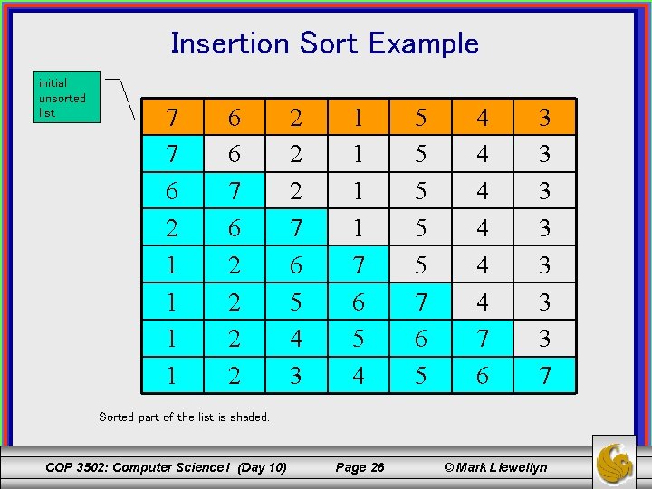
Insertion Sort Example initial unsorted list 7 7 6 2 1 1 6 6 7 6 2 2 2 2 7 6 5 4 3 1 1 7 6 5 4 5 5 5 7 6 5 4 4 4 7 6 3 3 3 3 7 Sorted part of the list is shaded. COP 3502: Computer Science I (Day 10) Page 26 © Mark Llewellyn

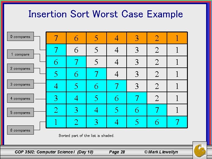
Worst Case Analysis for Insertion Sort • Look at the inner while loop of the algorithm. The most work this loop will do is when the new element to be added is smaller than all of the elements already in the sorted part of the list. In this situation, the loop will stop when the location becomes 0. • So, the most work the entire algorithm will do is in the case where every new element is added to the front of the list. For this case to occur, the list must be in decreasing order when the algorithm begins. • The next page illustrates this worst-case scenario. COP 3502: Computer Science I (Day 10) Page 27 © Mark Llewellyn

Insertion Sort Worst Case Example 0 compares 1 compare 2 compares 3 compares 4 compares 5 compares 7 7 6 5 4 3 2 1 6 6 7 6 5 4 3 2 5 5 5 7 6 5 4 3 4 4 7 6 5 4 3 3 3 7 6 5 2 2 2 7 6 1 1 1 1 7 6 compares Sorted part of the list is shaded. COP 3502: Computer Science I (Day 10) Page 28 © Mark Llewellyn

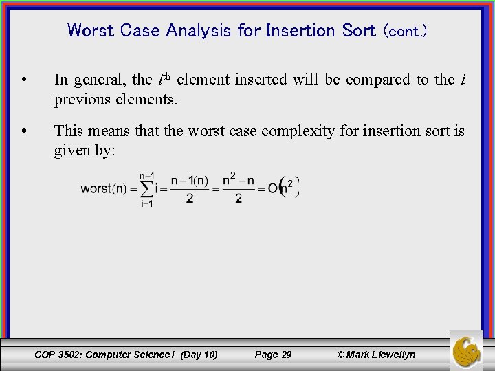
Worst Case Analysis for Insertion Sort (cont. ) • In general, the ith element inserted will be compared to the i previous elements. • This means that the worst case complexity for insertion sort is given by: COP 3502: Computer Science I (Day 10) Page 29 © Mark Llewellyn

Average Case Analysis for Insertion Sort • Average case analysis is a two-step process. First, we need to determine the average number of comparisons needed to move one element into place. Then, as a second step, we can determine the overall average number of operations by using the first step result for all of the other elements. • First, determine on average how many comparisons it takes to move the ith element into position. • We’ve already noted that adding the ith element to the sorted part of the list requires at most i comparisons. Obviously, one comparison is required even if the element remains in its current position. • How many different positions is it possible to move the ith element into? COP 3502: Computer Science I (Day 10) Page 30 © Mark Llewellyn

Average Case Analysis for Insertion Sort (cont. ) • Let’s look at small cases to see if we can identify a pattern that we can generalize. • There are two possibilities for the first element to be added, either location 1 or location 2. There are three possible locations for the second element to be added – either location 1, 2, or 3. • Thus, there are i+1 locations for the ith element. We’ll assume equal probability for all of these locations. • Now for the second part of the analysis. How many comparisons does it take to get to each of these i+1 possible locations? COP 3502: Computer Science I (Day 10) Page 31 © Mark Llewellyn

Average Case Analysis for Insertion Sort (cont. ) • Again, let’s consider small cases to see if we can identify a pattern that we can generalize. • If we are adding the fourth element, and it goes into location 5, the first comparison would fail. If it goes into location 4, the first comparison would succeed, but the second will fail. If it goes into location 3, the first two comparisons would succeed, but the third will fail. If it goes into location 2, the first three comparisons succeed and the fourth fails. If it goes into location 1, the first four comparisons succeed and there will be no further comparisons because the location will have become zero. • This implies that the ith element will require 1, 2, 3, …, i comparisons for locations i+1, i, i-1, …, 2, and will require i comparisons for location 1. COP 3502: Computer Science I (Day 10) Page 32 © Mark Llewellyn

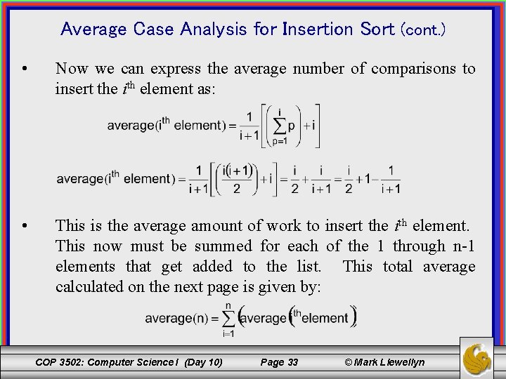
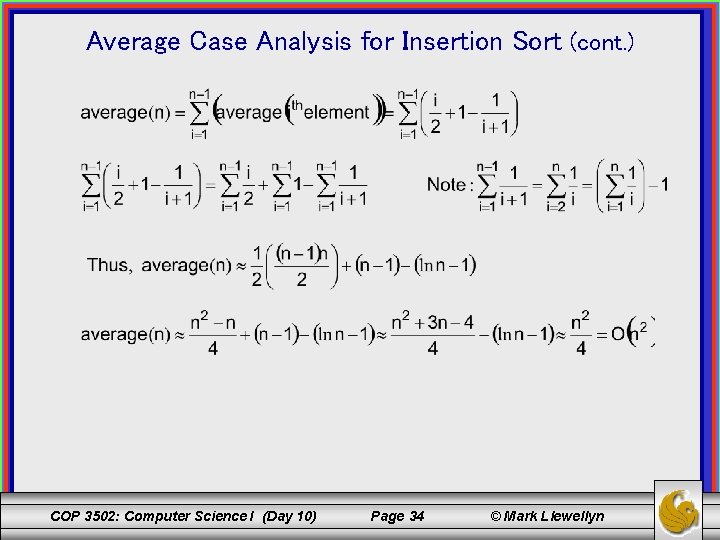
Average Case Analysis for Insertion Sort (cont. ) • Now we can express the average number of comparisons to insert the ith element as: • This is the average amount of work to insert the ith element. This now must be summed for each of the 1 through n-1 elements that get added to the list. This total average calculated on the next page is given by: COP 3502: Computer Science I (Day 10) Page 33 © Mark Llewellyn

Average Case Analysis for Insertion Sort (cont. ) COP 3502: Computer Science I (Day 10) Page 34 © Mark Llewellyn

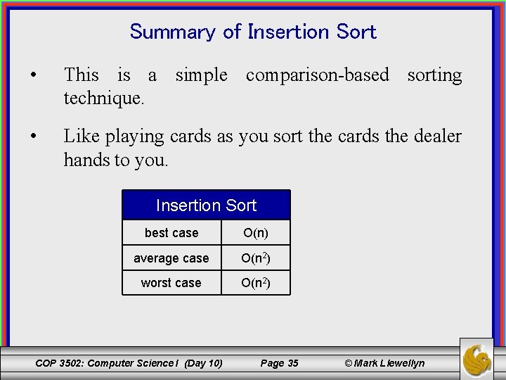
Summary of Insertion Sort • This is a simple comparison-based sorting technique. • Like playing cards as you sort the cards the dealer hands to you. Insertion Sort best case O(n) average case O(n 2) worst case O(n 2) COP 3502: Computer Science I (Day 10) Page 35 © Mark Llewellyn