COP 3502 Computer Science I Spring 2004 Note

COP 3502: Computer Science I Spring 2004 – Note Set 25 – Graphs – Part 3 Instructor : Mark Llewellyn markl@cs. ucf. edu CC 1 211, 823 -2790 http: //www. cs. ucf. edu/courses/cop 3502/spr 04 School of Electrical Engineering and Computer Science University of Central Florida COP 3502: Computer Science I (Note Set #25) Page 1 © Mark Llewellyn

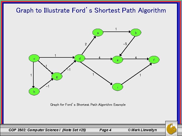
Ford’s Label Correcting Shortest Path Algorithm • One of the first label-correcting algorithms was developed by Lester Ford’s algorithm is more powerful than Dijkstra’s in that it can handle graphs with negative weights (but it cannot handle graphs with negative weight cycles). • To impose a certain ordering on monitoring the edges, an alphabetically ordered sequence of edges is commonly used so that the algorithm can repeatedly go through the entire sequence and adjust the current distance of any vertex if it is needed. • The graph shown on slide 4 contains negatively weighted edges but no negative weight cycles. COP 3502: Computer Science I (Note Set #25) Page 2 © Mark Llewellyn

Ford’s Label Correcting Shortest Path Algorithm (cont. ) • TAs with Dijkstra’s algorithm, Ford’s shortest path algorithm also uses a table. • We’ll run through an example like we did with Dijkstra’s algorithm so that you can get the feel for how this algorithm operates. • We’ll examine the table at each iteration of Ford’s algorithm as the while loop updates the current distances (one iteration is one pass through the edge set). • Note that a vertex can change its current distance during the same iteration. However, at the end, each vertex of the graph can be reached through the shortest path from the starting vertex. • The example assumes that the initial vertex was vertex c. COP 3502: Computer Science I (Note Set #25) Page 3 © Mark Llewellyn

Graph to Illustrate Ford’s Shortest Path Algorithm 1 a b 5 2 1 c 1 1 4 d e 4 f 1 g 1 1 1 i h Graph for Ford’s Shortest Path Algorithm Example COP 3502: Computer Science I (Note Set #25) Page 4 © Mark Llewellyn

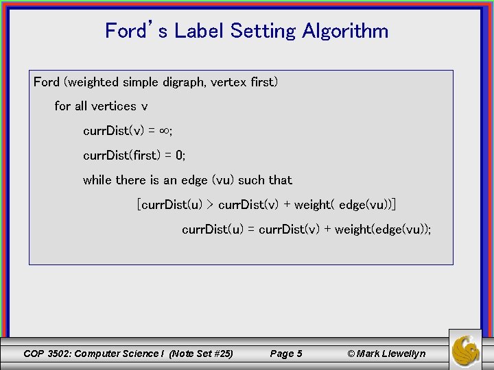
Ford’s Label Setting Algorithm Ford (weighted simple digraph, vertex first) for all vertices v curr. Dist(v) = ; curr. Dist(first) = 0; while there is an edge (vu) such that [curr. Dist(u) > curr. Dist(v) + weight( edge(vu))] curr. Dist(u) = curr. Dist(v) + weight(edge(vu)); COP 3502: Computer Science I (Note Set #25) Page 5 © Mark Llewellyn

Ford’s Label Correcting Shortest Path Algorithm (cont. ) • Notice that Ford’s algorithm does not specify the order in which the edges are checked. In the example, we will use the simple, but very brute force technique, of simply checking the adjacency list for every vertex during every iteration. This is not necessary and can be done much more efficiently, but clarity suffers and we are not worried about efficiency at this point. • Therefore, in the example the edges have been ordered alphabetically based upon the vertex letter. So, the edges are examined in the order of ab, be, cd, cg, ch, da, de, di, ef, gd, hg, if. Ford’s algorithm proceeds in much the same way that Dijkstra’s algorithm operates, however, termination occurs not when all vertices have been removed from a set but rather when no more changes (based upon the edge weights) can be made to any curr. Dist( ) value. • The next several slides illustrate the operation of Ford’s algorithm for the negatively weighted digraph on slide 4. COP 3502: Computer Science I (Note Set #25) Page 6 © Mark Llewellyn

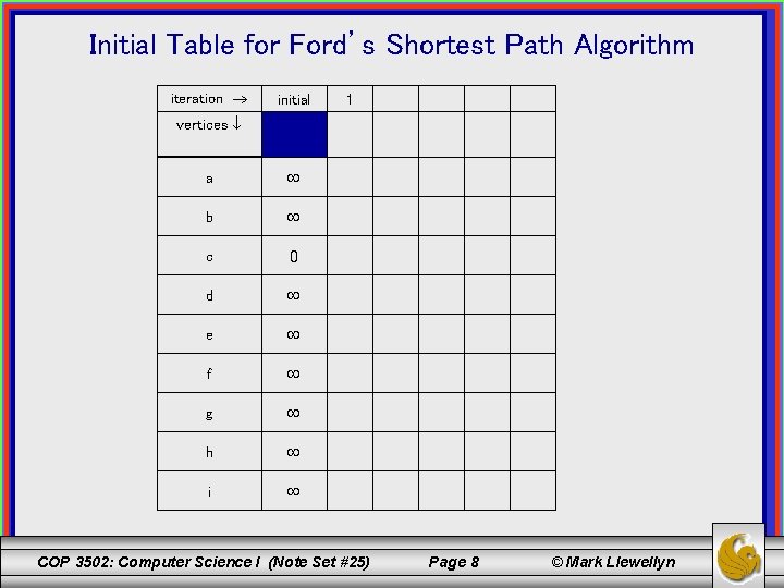
Initial Table for Ford’s Algorithm • Initially the curr. Dist(v) for every vertex in the graph is set to . • Next the curr. Dist(start) is set to 0, where start is the initial node for the path. – In this example start = vertex c. • Edge ordering is: ab, be, cd, cg, ch, da, de, di, ef, gd, hg, if. • The initial table is shown on the next slide. COP 3502: Computer Science I (Note Set #25) Page 7 © Mark Llewellyn

Initial Table for Ford’s Shortest Path Algorithm iteration initial 1 vertices a b c 0 d e f g h i COP 3502: Computer Science I (Note Set #25) Page 8 © Mark Llewellyn

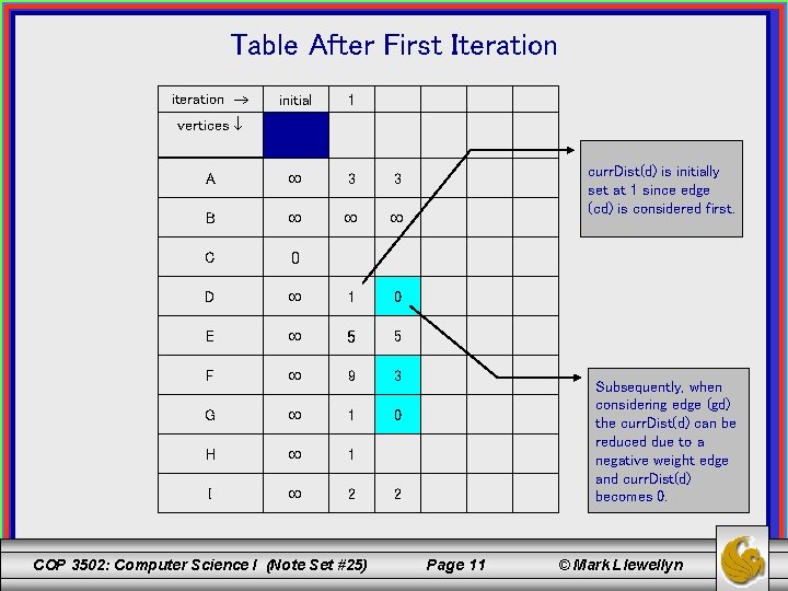
First Iteration of Ford’s Algorithm • Since the edge set is ordered alphabetically and we are assuming that the start vertex is c, then the first iteration of the while loop in the algorithm will ignore the first two edges (ab) and (be). • The first past will set the curr. Dist( ) value for all single edge paths (at least), the second pass will set all the values for two-edge paths, and so on. • In this example graph the longest path is of length four so only four iterations will be required to determine the shortest path from vertex c to all other vertices. • The table on slide 11 shows the status after the first iteration completes. Notice that the path from c to d is reset (as are the paths from c to f and c to g) since a path of two edges has less weight than the first path of one edge. This is illustrated in the un-numbered (un-labeled) column. COP 3502: Computer Science I (Note Set #25) Page 9 © Mark Llewellyn

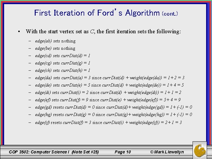
First Iteration of Ford’s Algorithm (cont. ) • With the start vertex set as C, the first iteration sets the following: – edge(ab) sets nothing – edge(be) sets nothing – edge(cd) sets curr. Dist(d) = 1 – edge(cg) sets curr. Dist(g) = 1 – edge(ch) sets curr. Dist(h) = 1 – edge(da) sets curr. Dist(a) = 3 since curr. Dist(d) + weight(edge(da)) = 1+ 2 = 3 – edge(de) sets curr. Dist(e) = 5 since curr. Dist(d) + weight(edge(de)) = 1+ 4 = 5 – edge(di) sets curr. Dist(i) = 2 since curr. Dist(d) + weight(edge(di)) = 1+ 1 = 2 – edge(ef) sets curr. Dist(f) = 9 since curr. Dist(e) + weight(edge(ef)) = 5+ 4 = 9 – edge(gd) resets curr. Dist(d) = 0 since curr. Dist(d)+ weight(edge(gd)) = 1+ (-1) = 0 – edge(hg) resets curr. Dist(g) = 0 since curr. Dist(g)+ weight(edge(hg)) = 1+ (-1) = 0 – edge(if) resets curr. Dist(f) = 3 since curr. Dist(i) + weight(edge(if)) = 2+ 1 = 3 COP 3502: Computer Science I (Note Set #25) Page 10 © Mark Llewellyn

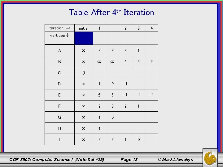
Table After First Iteration iteration initial 1 A 3 3 B C 0 D 1 0 E 5 5 F 9 3 G 1 0 H 1 I 2 vertices COP 3502: Computer Science I (Note Set #25) curr. Dist(d) is initially set at 1 since edge (cd) is considered first. Subsequently, when considering edge (gd) the curr. Dist(d) can be reduced due to a negative weight edge and curr. Dist(d) becomes 0. 2 Page 11 © Mark Llewellyn

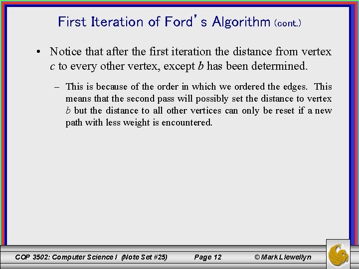
First Iteration of Ford’s Algorithm (cont. ) • Notice that after the first iteration the distance from vertex c to every other vertex, except b has been determined. – This is because of the order in which we ordered the edges. This means that the second pass will possibly set the distance to vertex b but the distance to all other vertices can only be reset if a new path with less weight is encountered. COP 3502: Computer Science I (Note Set #25) Page 12 © Mark Llewellyn

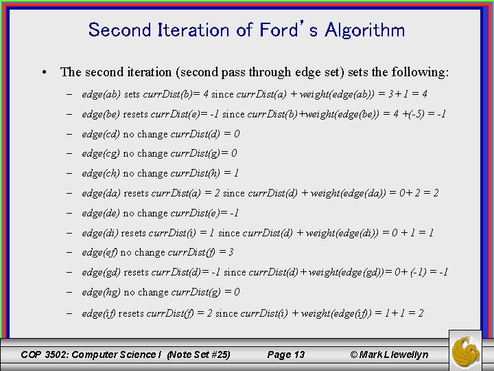
Second Iteration of Ford’s Algorithm • The second iteration (second pass through edge set) sets the following: – edge(ab) sets curr. Dist(b)= 4 since curr. Dist(a) + weight(edge(ab)) = 3+ 1 = 4 – edge(be) resets curr. Dist(e)= -1 since curr. Dist(b)+weight(edge(be)) = 4 +(-5) = -1 – edge(cd) no change curr. Dist(d) = 0 – edge(cg) no change curr. Dist(g)= 0 – edge(ch) no change curr. Dist(h) = 1 – edge(da) resets curr. Dist(a) = 2 since curr. Dist(d) + weight(edge(da)) = 0+ 2 = 2 – edge(de) no change curr. Dist(e)= -1 – edge(di) resets curr. Dist(i) = 1 since curr. Dist(d) + weight(edge(di)) = 0 + 1 = 1 – edge(ef) no change curr. Dist(f) = 3 – edge(gd) resets curr. Dist(d)= -1 since curr. Dist(d)+ weight(edge(gd))= 0+ (-1) = -1 – edge(hg) no change curr. Dist(g) = 0 – edge(if) resets curr. Dist(f) = 2 since curr. Dist(i) + weight(edge(if)) = 1+ 1 = 2 COP 3502: Computer Science I (Note Set #25) Page 13 © Mark Llewellyn

Table After 2 nd Iteration iteration initial 1 2 A 3 3 2 B 4 C 0 D 1 0 1 E 5 5 1 F 9 3 2 G 1 0 H 1 I 2 vertices COP 3502: Computer Science I (Note Set #25) 2 1 Page 14 © Mark Llewellyn

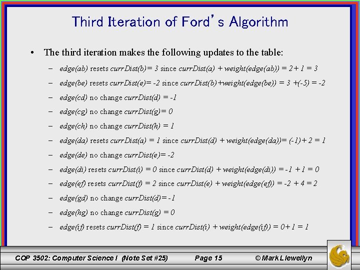
Third Iteration of Ford’s Algorithm • The third iteration makes the following updates to the table: – edge(ab) resets curr. Dist(b)= 3 since curr. Dist(a) + weight(edge(ab)) = 2+ 1 = 3 – edge(be) resets curr. Dist(e)= -2 since curr. Dist(b)+weight(edge(be)) = 3 +(-5) = -2 – edge(cd) no change curr. Dist(d) = -1 – edge(cg) no change curr. Dist(g)= 0 – edge(ch) no change curr. Dist(h) = 1 – edge(da) resets curr. Dist(a) = 1 since curr. Dist(d) + weight(edge(da))= (-1)+ 2 = 1 – edge(de) no change curr. Dist(e)= -2 – edge(di) resets curr. Dist(i) = 0 since curr. Dist(d) + weight(edge(di)) = -1 + 1 = 0 – edge(ef) resets curr. Dist(f) = 2 since curr. Dist(e) + weight(edge(ef)) = -2 + 4 = 2 – edge(gd) no change curr. Dist(d)= -1 – edge(hg) no change curr. Dist(g) = 0 – edge(if) resets curr. Dist(f) = 1 since curr. Dist(i) + weight(edge(if)) = 0+ 1 = 1 COP 3502: Computer Science I (Note Set #25) Page 15 © Mark Llewellyn

Table After 3 rd Iteration iteration initial 1 2 3 A 3 3 2 1 B 4 3 C 0 D 1 0 1 E 5 5 1 2 F 9 3 2 1 G 1 0 H 1 I 2 1 0 vertices COP 3502: Computer Science I (Note Set #25) 2 Page 16 © Mark Llewellyn

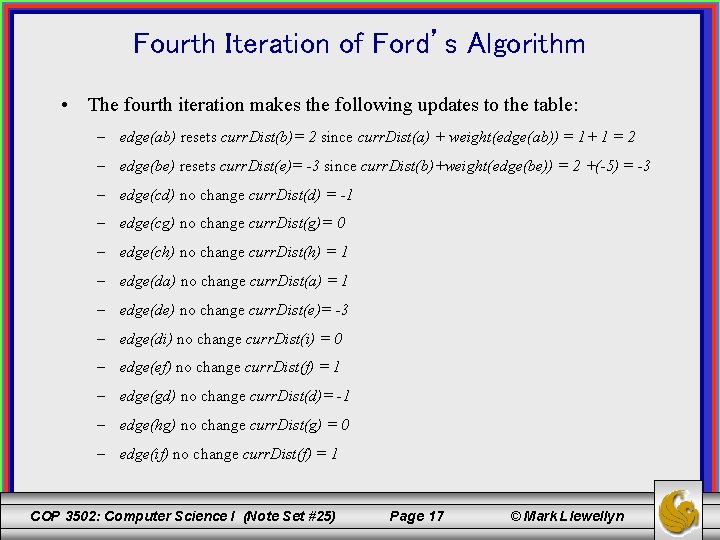
Fourth Iteration of Ford’s Algorithm • The fourth iteration makes the following updates to the table: – edge(ab) resets curr. Dist(b)= 2 since curr. Dist(a) + weight(edge(ab)) = 1+ 1 = 2 – edge(be) resets curr. Dist(e)= -3 since curr. Dist(b)+weight(edge(be)) = 2 +(-5) = -3 – edge(cd) no change curr. Dist(d) = -1 – edge(cg) no change curr. Dist(g)= 0 – edge(ch) no change curr. Dist(h) = 1 – edge(da) no change curr. Dist(a) = 1 – edge(de) no change curr. Dist(e)= -3 – edge(di) no change curr. Dist(i) = 0 – edge(ef) no change curr. Dist(f) = 1 – edge(gd) no change curr. Dist(d)= -1 – edge(hg) no change curr. Dist(g) = 0 – edge(if) no change curr. Dist(f) = 1 COP 3502: Computer Science I (Note Set #25) Page 17 © Mark Llewellyn

Table After 4 th Iteration iteration initial 1 2 3 A 3 B C 0 D 4 3 2 1 0 1 E 5 5 1 2 3 F 9 3 2 1 G 1 0 H 1 I 2 1 0 vertices COP 3502: Computer Science I (Note Set #25) 2 Page 18 © Mark Llewellyn

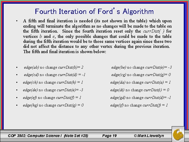
Fourth Iteration of Ford’s Algorithm • A fifth and final iteration is needed (its not shown in the table) which upon ending will terminate the algorithm as no changes will be made to the table on the fifth iteration. Since the fourth iteration reset only the curr. Dist( ) for vertices b and e, the only possible changes that could be made to the table during the fifth iteration would be to those same vertices again since these two did not affect the distance to any other vertex during the previous iteration. The fifth and final iteration is shown below: • edge(ab) no change curr. Dist(b)= 2 edge(be) no change curr. Dist(e)= -3 • edge(cd) no change curr. Dist(d) = -1 edge(cg) no change curr. Dist(g)= 0 • edge(ch) no change curr. Dist(h) = 1 edge(da) no change curr. Dist(a) = 1 • edge(de) no change curr. Dist(e)= -3 edge(di) no change curr. Dist(i) = 0 • edge(ef) no change curr. Dist(f) = 1 edge(gd) no change curr. Dist(d)= -1 • edge(hg) no change curr. Dist(g) = 0 edge(if) no change curr. Dist(f) = 1 COP 3502: Computer Science I (Note Set #25) Page 19 © Mark Llewellyn

Comments on Ford’s Shortest Path Algorithm • As you can see having stepped through the execution of Ford’s algorithm, the run-time is dependent on the size of the edge set. • Ford’s algorithm works best if the graph is sparse and less well if the graph is relatively dense. COP 3502: Computer Science I (Note Set #25) Page 20 © Mark Llewellyn