COP 3502 Computer Science I Spring 2004 Day

COP 3502: Computer Science I Spring 2004 – Day 7 – Algorithm Analysis Instructor : Mark Llewellyn markl@cs. ucf. edu CC 1 211, 823 -2790 http: //www. cs. ucf. edu/courses/cop 3502/spr 04 School of Electrical Engineering and Computer Science University of Central Florida COP 3502: Computer Science I (Day 7) Page 1 Mark Llewellyn

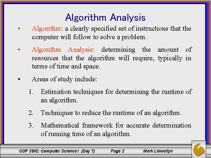
Algorithm Analysis • Algorithm: a clearly specified set of instructions that the computer will follow to solve a problem. • Algorithm Analysis: determining the amount of resources that the algorithm will require, typically in terms of time and space. • Areas of study include: 1. Estimation techniques for determining the runtime of an algorithm. 2. Techniques to reduce the runtime of an algorithm. 3. Mathematical framework for accurate determination of running time of an algorithm. COP 3502: Computer Science I (Day 7) Page 2 Mark Llewellyn

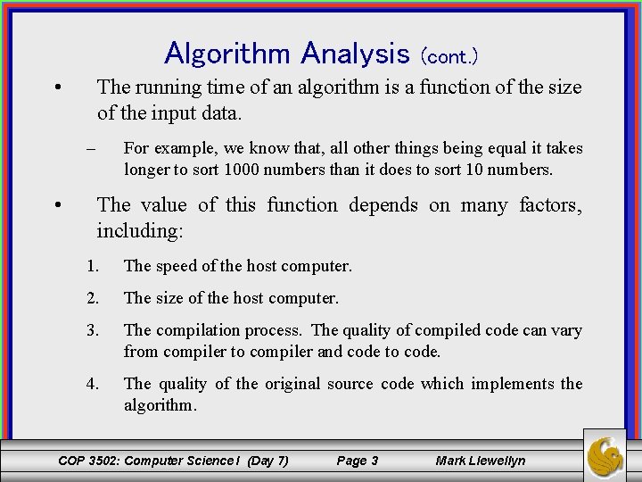
Algorithm Analysis (cont. ) The running time of an algorithm is a function of the size of the input data. • – • For example, we know that, all other things being equal it takes longer to sort 1000 numbers than it does to sort 10 numbers. The value of this function depends on many factors, including: 1. The speed of the host computer. 2. The size of the host computer. 3. The compilation process. The quality of compiled code can vary from compiler to compiler and code to code. 4. The quality of the original source code which implements the algorithm. COP 3502: Computer Science I (Day 7) Page 3 Mark Llewellyn

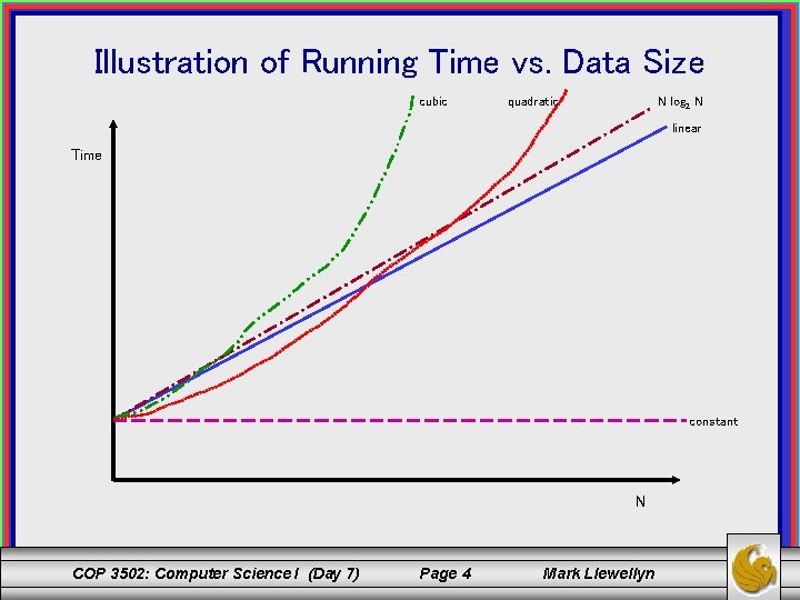
Illustration of Running Time vs. Data Size cubic N log 2 N quadratic linear Time constant N COP 3502: Computer Science I (Day 7) Page 4 Mark Llewellyn

Comparing Functions • When comparing two functions F(N) and G(N), it does not make sense to state that: F < G, F = G, or G < F. – Example: At some arbitrary point x, F may be smaller than G, yet at some other point y, F may be equal to or greater than G. • Instead, the growth rates of the functions need to be determined. • There is a three-fold reason for basing our analysis on the growth rate of the function rather than its specific value at some point: COP 3502: Computer Science I (Day 7) Page 5 Mark Llewellyn

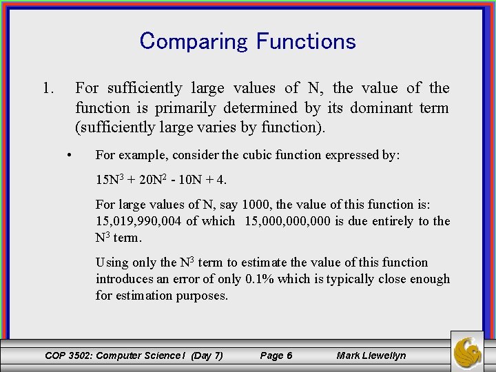
Comparing Functions 1. For sufficiently large values of N, the value of the function is primarily determined by its dominant term (sufficiently large varies by function). • For example, consider the cubic function expressed by: 15 N 3 + 20 N 2 - 10 N + 4. For large values of N, say 1000, the value of this function is: 15, 019, 990, 004 of which 15, 000, 000 is due entirely to the N 3 term. Using only the N 3 term to estimate the value of this function introduces an error of only 0. 1% which is typically close enough for estimation purposes. COP 3502: Computer Science I (Day 7) Page 6 Mark Llewellyn

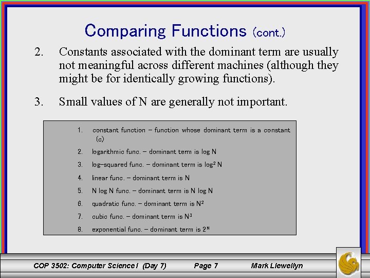
Comparing Functions (cont. ) 2. Constants associated with the dominant term are usually not meaningful across different machines (although they might be for identically growing functions). 3. Small values of N are generally not important. 1. constant function – function whose dominant term is a constant (c) 2. logarithmic func. – dominant term is log N 3. log-squared func. – dominant term is log 2 N 4. linear func. – dominant term is N 5. N log N func. – dominant term is N log N 6. quadratic func. – dominant term is N 2 7. cubic func. – dominant term is N 3 8. exponential func. – dominant term is 2 N COP 3502: Computer Science I (Day 7) Page 7 Mark Llewellyn

Measures of Work • Evaluating and comparing the work required by various algorithms is an important component of software engineering. • In fact, it is only by such measures that we can identify which of various possible algorithms for a given problem is preferable. • In general, there are three different metrics by which algorithms are evaluated: 1. Best case 2. Worst case 3. Average case COP 3502: Computer Science I (Day 7) Page 8 Mark Llewellyn

Measures of Work (cont. ) • Consider the following problem: I give you a set of eight coins and a comparator scale (gives relative not absolute weights). I tell you that one of the coins maybe counterfeit and that counterfeit coins weigh less than real coins. Your mission (should you decide to accept it) is to determine if the set of coins contains a counterfeit coin. • Question: In terms of the number of comparisons which are necessary what is the best case, worst case, and average case for this problem? COP 3502: Computer Science I (Day 7) Page 9 Mark Llewellyn

Measures of Work (cont. ) • Consider the following problem: I give you a set of eight coins and a comparator scale (gives relative not absolute weights). I tell you that one of the coins maybe counterfeit and that counterfeit coins weigh less than real coins. Your mission (should you decide to accept it) is to determine if the set of coins contains a counterfeit coin. • Question: In terms of the number of comparisons which are necessary what is the best case, worst case, and average case for this problem? COP 3502: Computer Science I (Day 7) Page 10 Mark Llewellyn

Measures of Work (cont. ) • First, you need to devise an algorithm that will solve the problem. • Let’s use the following algorithm: divide the set of 8 coins into 4 sets of two coins each. Put a pair of coins on the scale and compare their weights. If they are different, stop – counterfeit coin detected; otherwise, repeat process until all coins have been compared, stop – no counterfeit coin detected. COP 3502: Computer Science I (Day 7) Page 11 Mark Llewellyn

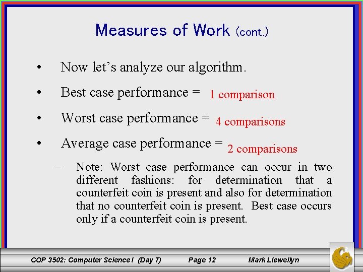
Measures of Work (cont. ) • Now let’s analyze our algorithm. • Best case performance = 1 comparison • Worst case performance = 4 comparisons • Average case performance = 2 comparisons – Note: Worst case performance can occur in two different fashions: for determination that a counterfeit coin is present and also for determination that no counterfeit coin is present. Best case occurs only if a counterfeit coin is present. COP 3502: Computer Science I (Day 7) Page 12 Mark Llewellyn

Measures of Work (cont. ) • The obvious question at this point is, “can we do better? ” • What do we mean by “better”? • Better best case? Better worst case? Better average case? Better for all three? • Sometimes improving one, improves the others. • For the algorithm that we started with, the answer is no, we cannot do any “better” in terms of reducing the number of comparisons in either the best, worst, or average cases. • Let’s try another algorithm. COP 3502: Computer Science I (Day 7) Page 13 Mark Llewellyn

Measures of Work (cont. ) • Can you think of a different algorithm to solve this problem? • How about this one: divide the set of 8 coins into 2 sets of four coins each. Put both sets of coins on the scale and compare their weights. If they are different, stop – counterfeit coin detected; otherwise, stop – no counterfeit coin detected. COP 3502: Computer Science I (Day 7) Page 14 Mark Llewellyn

Measures of Work (cont. ) • Now let’s analyze our new algorithm. • Best case performance = 1 comparison • Worst case performance = 1 comparison • Average case performance = 1 comparison Clearly our new algorithm is “better” since both the worst case and the average case performance require fewer comparisons (our metric in this example). COP 3502: Computer Science I (Day 7) Page 15 Mark Llewellyn

Measures of Work (cont. ) • Now let’s’ slightly modify the original problem to the following: I give you a set of eight coins and a comparator scale (gives relative not absolute weights). I tell you that one of the coins maybe counterfeit and that counterfeit coins weigh less than real coins. Your mission now is to identify the counterfeit coin if one exists in the set. • Question: Once again, we’ll analyze our algorithm in terms of the number of comparisons which are necessary what is the best case, worst case, and average case for this problem? COP 3502: Computer Science I (Day 7) Page 16 Mark Llewellyn

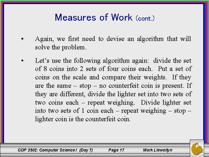
Measures of Work (cont. ) • Again, we first need to devise an algorithm that will solve the problem. • Let’s use the following algorithm again: divide the set of 8 coins into 2 sets of four coins each. Put a set of coins on the scale and compare their weights. If they are the same – stop – no counterfeit coin is present. If they are different, divide the lighter set into two sets of two coins each – repeat weighing. Divide lighter set into two sets of 1 coin each – repeat weighing – stop – lighter coin is the counterfeit coin. COP 3502: Computer Science I (Day 7) Page 17 Mark Llewellyn

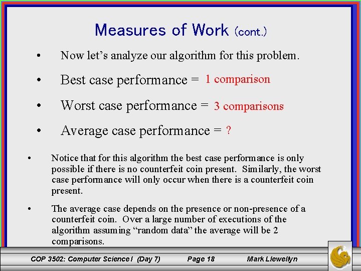
Measures of Work (cont. ) • Now let’s analyze our algorithm for this problem. • Best case performance = 1 comparison • Worst case performance = 3 comparisons • Average case performance = ? • Notice that for this algorithm the best case performance is only possible if there is no counterfeit coin present. Similarly, the worst case performance will only occur when there is a counterfeit coin present. • The average case depends on the presence or non-presence of a counterfeit coin. Over a large number of executions of the algorithm assuming “random data” the average will be 2 comparisons. COP 3502: Computer Science I (Day 7) Page 18 Mark Llewellyn

Random Data • The discussion of the average number of comparisons made by our counterfeit coin detector algorithm brings up an important issue in algorithm analysis. • What do we mean when we say that the input data is “random” or “average”? • How does “random” or “average” data compare with the “actual” data that we would expect to see at run-time? COP 3502: Computer Science I (Day 7) Page 19 Mark Llewellyn

Random Data (cont. ) • It turns out that in many instances, the assumption that the input data to an algorithm is random, is a faulty assumption. • In order to truly get a handle on what constitutes “average input” we need to be alert to any properties of the data or of the operational situation in which the algorithm will be executed that will impact what constitutes the average case. COP 3502: Computer Science I (Day 7) Page 20 Mark Llewellyn

Random Data (cont. ) • Consider the following case: When the phone company produces a new phone book for the Orlando area, it clearly needs to sort the names that will appear in the new version of the phone book in alphabetical order. • Does the input to the phone book sorting algorithm appear as random data? Obviously not, they do not resort the entire listing of names that already appear in the phonebook. Rather they merge the new names into the existing names to create one giant sorted set of names. • In other words, most of the data that is being sorted, is in fact already sorted. This is clearly different than truly random data and will obviously impact the sort time. COP 3502: Computer Science I (Day 7) Page 21 Mark Llewellyn

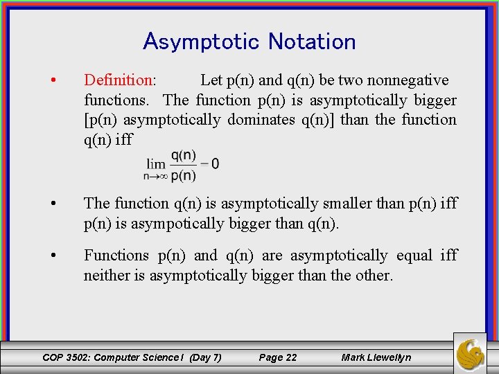
Asymptotic Notation • Definition: Let p(n) and q(n) be two nonnegative functions. The function p(n) is asymptotically bigger [p(n) asymptotically dominates q(n)] than the function q(n) iff • The function q(n) is asymptotically smaller than p(n) iff p(n) is asympotically bigger than q(n). • Functions p(n) and q(n) are asymptotically equal iff neither is asymptotically bigger than the other. COP 3502: Computer Science I (Day 7) Page 22 Mark Llewellyn

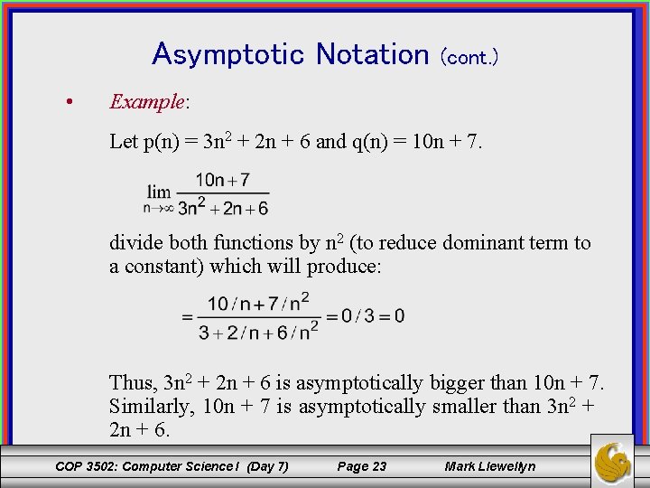
Asymptotic Notation • (cont. ) Example: Let p(n) = 3 n 2 + 2 n + 6 and q(n) = 10 n + 7. divide both functions by n 2 (to reduce dominant term to a constant) which will produce: Thus, 3 n 2 + 2 n + 6 is asymptotically bigger than 10 n + 7. Similarly, 10 n + 7 is asymptotically smaller than 3 n 2 + 2 n + 6. COP 3502: Computer Science I (Day 7) Page 23 Mark Llewellyn

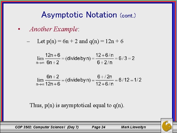
Asymptotic Notation • (cont. ) Another Example: – Let p(n) = 6 n + 2 and q(n) = 12 n + 6 Thus, p(n) is asymptotical equal to q(n). COP 3502: Computer Science I (Day 7) Page 24 Mark Llewellyn

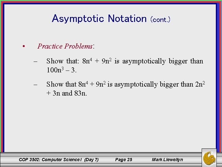
Asymptotic Notation • (cont. ) Practice Problems: – Show that: 8 n 4 + 9 n 2 is asymptotically bigger than 100 n 3 – 3. – Show that 8 n 4 + 9 n 2 is asymptotically bigger than 2 n 2 + 3 n and 83 n. COP 3502: Computer Science I (Day 7) Page 25 Mark Llewellyn

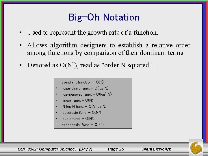
Big-Oh Notation • Used to represent the growth rate of a function. • Allows algorithm designers to establish a relative order among functions by comparison of their dominant terms. • Denoted as O(N 2), read as "order N squared". • • constant function – O(1) logarithmic func. – O(log N) log-squared func. – O(log 2 N) linear func. – O(N) N log N func. – O(N log N) quadratic func. – O(N 2) cubic func. – O(N 3) exponential func. – O(2 N) COP 3502: Computer Science I (Day 7) Page 26 Mark Llewellyn

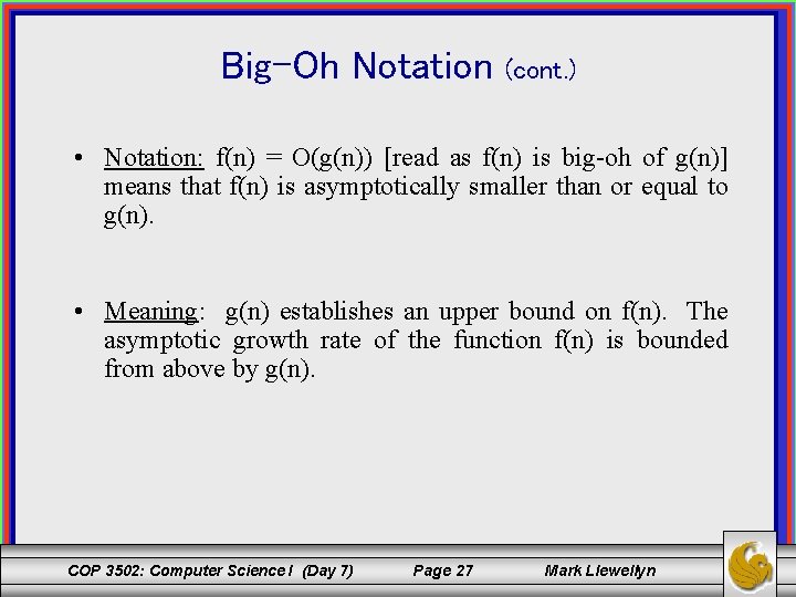
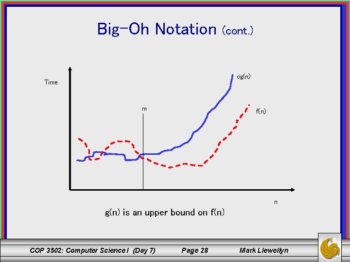
Big-Oh Notation (cont. ) • Notation: f(n) = O(g(n)) [read as f(n) is big-oh of g(n)] means that f(n) is asymptotically smaller than or equal to g(n). • Meaning: g(n) establishes an upper bound on f(n). The asymptotic growth rate of the function f(n) is bounded from above by g(n). COP 3502: Computer Science I (Day 7) Page 27 Mark Llewellyn

Big-Oh Notation (cont. ) cg(n) Time m f(n) n g(n) is an upper bound on f(n) COP 3502: Computer Science I (Day 7) Page 28 Mark Llewellyn