COP 3502 Computer Science I Spring 2004 Day

COP 3502: Computer Science I Spring 2004 – Day 8 – Algorithm Analysis – Part 2 Instructor : Mark Llewellyn markl@cs. ucf. edu CC 1 211, 823 -2790 http: //www. cs. ucf. edu/courses/cop 3502/spr 04 School of Electrical Engineering and Computer Science University of Central Florida COP 3502: Computer Science I (Day 8) Page 1 Mark Llewellyn

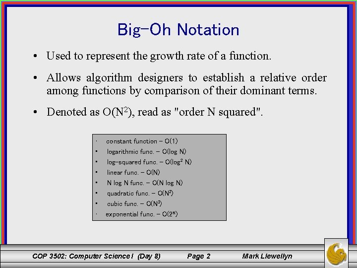
Big-Oh Notation • Used to represent the growth rate of a function. • Allows algorithm designers to establish a relative order among functions by comparison of their dominant terms. • Denoted as O(N 2), read as "order N squared". • • constant function – O(1) logarithmic func. – O(log N) log-squared func. – O(log 2 N) linear func. – O(N) N log N func. – O(N log N) quadratic func. – O(N 2) cubic func. – O(N 3) exponential func. – O(2 N) COP 3502: Computer Science I (Day 8) Page 2 Mark Llewellyn

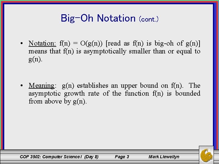
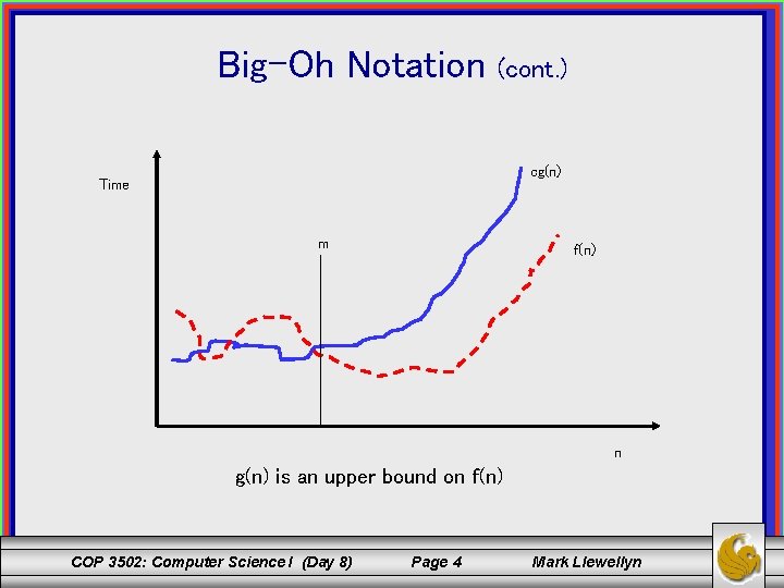
Big-Oh Notation (cont. ) • Notation: f(n) = O(g(n)) [read as f(n) is big-oh of g(n)] means that f(n) is asymptotically smaller than or equal to g(n). • Meaning: g(n) establishes an upper bound on f(n). The asymptotic growth rate of the function f(n) is bounded from above by g(n). COP 3502: Computer Science I (Day 8) Page 3 Mark Llewellyn

Big-Oh Notation (cont. ) cg(n) Time m f(n) n g(n) is an upper bound on f(n) COP 3502: Computer Science I (Day 8) Page 4 Mark Llewellyn

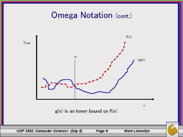
Omega Notation: f(n) = (g(n)) [read as f(n) is omega of g(n)] means that f(n) is asymptotically bigger than or equal to g(n). Meaning: g(n) establishes a lower bound on f(n). The asymptotic growth rate of the function f(n) is bounded from below by g(n). COP 3502: Computer Science I (Day 8) Page 5 Mark Llewellyn

Omega Notation (cont. ) f(n) Time m cg(n) n g(n) is an lower bound on f(n) COP 3502: Computer Science I (Day 8) Page 6 Mark Llewellyn

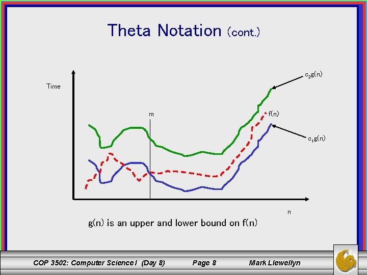
Theta Notation: f(n) = (g(n)) [read as f(n) is theta of g(n)] means that f(n) is asymptotically equal to g(n). Meaning: g(n) and f(n) have the same characteristics. COP 3502: Computer Science I (Day 8) Page 7 Mark Llewellyn

Theta Notation (cont. ) c 2 g(n) Time m f(n) c 1 g(n) n g(n) is an upper and lower bound on f(n) COP 3502: Computer Science I (Day 8) Page 8 Mark Llewellyn

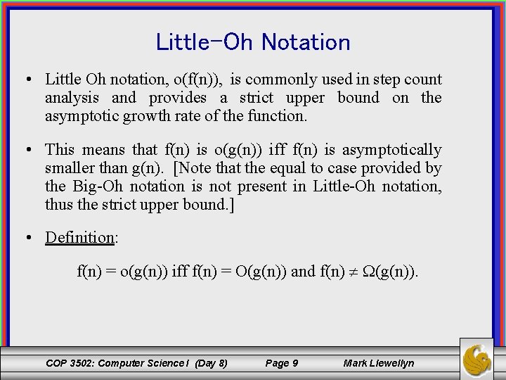
Little-Oh Notation • Little Oh notation, o(f(n)), is commonly used in step count analysis and provides a strict upper bound on the asymptotic growth rate of the function. • This means that f(n) is o(g(n)) iff f(n) is asymptotically smaller than g(n). [Note that the equal to case provided by the Big-Oh notation is not present in Little-Oh notation, thus the strict upper bound. ] • Definition: f(n) = o(g(n)) iff f(n) = O(g(n)) and f(n) (g(n)). COP 3502: Computer Science I (Day 8) Page 9 Mark Llewellyn

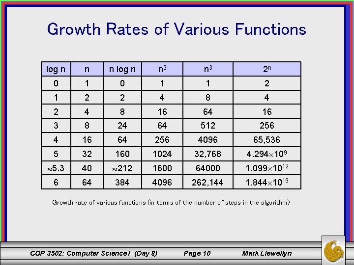
Growth Rates of Various Functions log n n n log n n 2 n 3 2 n 0 1 1 2 2 4 8 4 2 4 8 16 64 16 3 8 24 64 512 256 4 16 64 256 4096 65, 536 5 32 160 1024 32, 768 4. 294 109 5. 3 40 212 1600 64000 1. 099 1012 6 64 384 4096 262, 144 1. 844 1019 Growth rate of various functions (in terms of the number of steps in the algorithm) COP 3502: Computer Science I (Day 8) Page 10 Mark Llewellyn

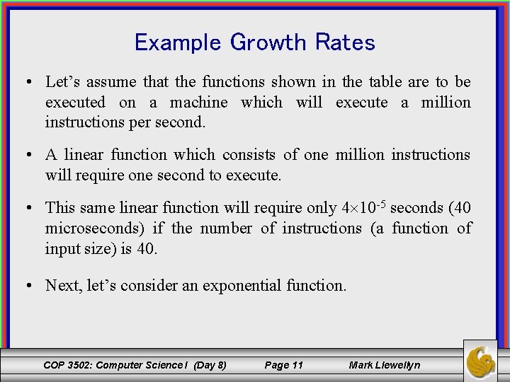
Example Growth Rates • Let’s assume that the functions shown in the table are to be executed on a machine which will execute a million instructions per second. • A linear function which consists of one million instructions will require one second to execute. • This same linear function will require only 4 10 -5 seconds (40 microseconds) if the number of instructions (a function of input size) is 40. • Next, let’s consider an exponential function. COP 3502: Computer Science I (Day 8) Page 11 Mark Llewellyn

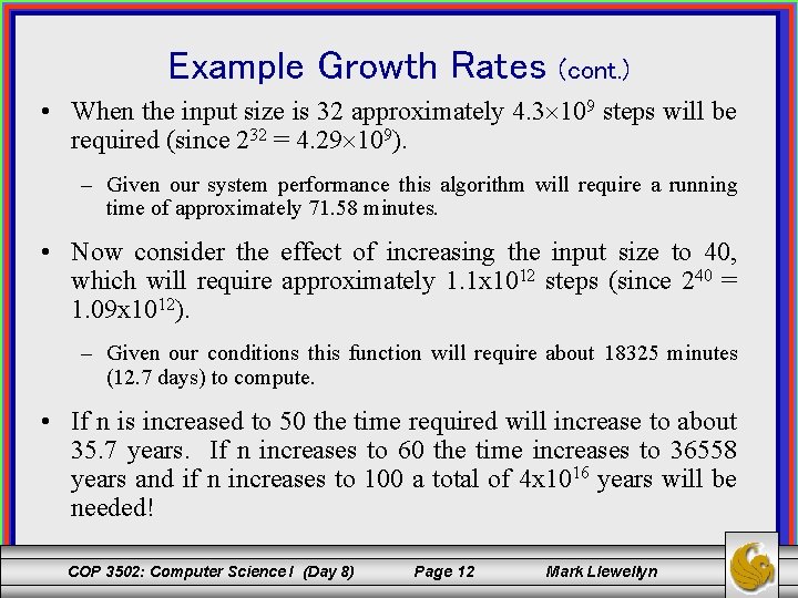
Example Growth Rates (cont. ) • When the input size is 32 approximately 4. 3 109 steps will be required (since 232 = 4. 29 109). – Given our system performance this algorithm will require a running time of approximately 71. 58 minutes. • Now consider the effect of increasing the input size to 40, which will require approximately 1. 1 x 1012 steps (since 240 = 1. 09 x 1012). – Given our conditions this function will require about 18325 minutes (12. 7 days) to compute. • If n is increased to 50 the time required will increase to about 35. 7 years. If n increases to 60 the time increases to 36558 years and if n increases to 100 a total of 4 x 1016 years will be needed! COP 3502: Computer Science I (Day 8) Page 12 Mark Llewellyn

Algorithm Analysis • Remember, that baring some type of looping statement, the code in a program (algorithm) is executed sequentially on von Neumann type architecture. • This means that without loops, each statement is executed exactly one time and the running time of the algorithm is very easy to establish. • Loops cause iteration and iteration increases the running time depending on how much iteration occurs. • Therefore, we need to know, for the statements inside the loop, how many times they are executed. COP 3502: Computer Science I (Day 8) Page 13 Mark Llewellyn

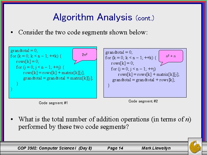
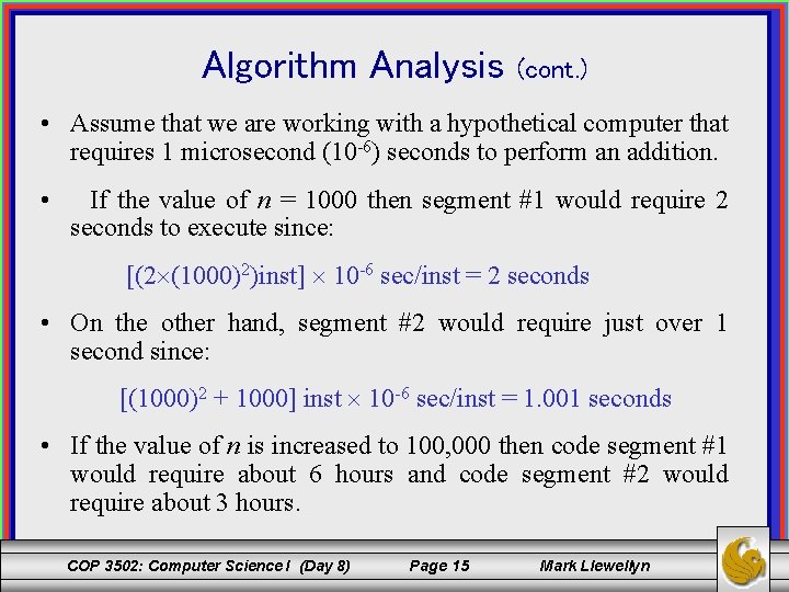
Algorithm Analysis (cont. ) • Consider the two code segments shown below: grandtotal = 0; 2 n 2 for (k = 0; k < n – 1; ++k) { rows[k] = 0; for (j = 0; j < n – 1; ++j) { rows[k] = rows[k] + matrix[k][j]; grandtotal = grandtotal + matrix[k][j]; } } grandtotal = 0; n 2 + n for (k = 0; k < n – 1; ++k) { rows[k] = 0; for (j = 0; j < n – 1; ++j) rows[k] = rows[k] + matrix[k][j]; grandtotal = grandtotal + rows]k]; } Code segment #2 Code segment #1 • What is the total number of addition operations (in terms of n) performed by these two code segments? COP 3502: Computer Science I (Day 8) Page 14 Mark Llewellyn

Algorithm Analysis (cont. ) • Assume that we are working with a hypothetical computer that requires 1 microsecond (10 -6) seconds to perform an addition. • If the value of n = 1000 then segment #1 would require 2 seconds to execute since: [(2 (1000)2)inst] 10 -6 sec/inst = 2 seconds • On the other hand, segment #2 would require just over 1 second since: [(1000)2 + 1000] inst 10 -6 sec/inst = 1. 001 seconds • If the value of n is increased to 100, 000 then code segment #1 would require about 6 hours and code segment #2 would require about 3 hours. COP 3502: Computer Science I (Day 8) Page 15 Mark Llewellyn

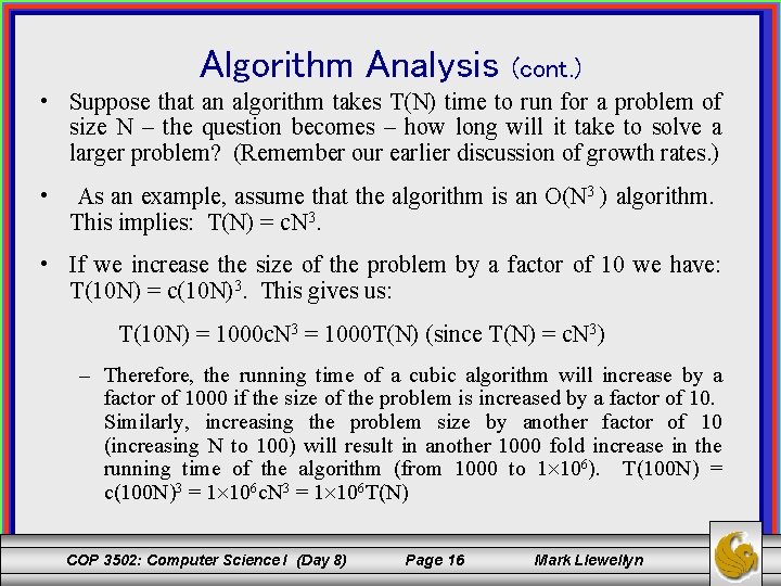
Algorithm Analysis (cont. ) • Suppose that an algorithm takes T(N) time to run for a problem of size N – the question becomes – how long will it take to solve a larger problem? (Remember our earlier discussion of growth rates. ) • As an example, assume that the algorithm is an O(N 3 ) algorithm. This implies: T(N) = c. N 3. • If we increase the size of the problem by a factor of 10 we have: T(10 N) = c(10 N)3. This gives us: T(10 N) = 1000 c. N 3 = 1000 T(N) (since T(N) = c. N 3) – Therefore, the running time of a cubic algorithm will increase by a factor of 1000 if the size of the problem is increased by a factor of 10. Similarly, increasing the problem size by another factor of 10 (increasing N to 100) will result in another 1000 fold increase in the running time of the algorithm (from 1000 to 1 106). T(100 N) = c(100 N)3 = 1 106 c. N 3 = 1 106 T(N) COP 3502: Computer Science I (Day 8) Page 16 Mark Llewellyn

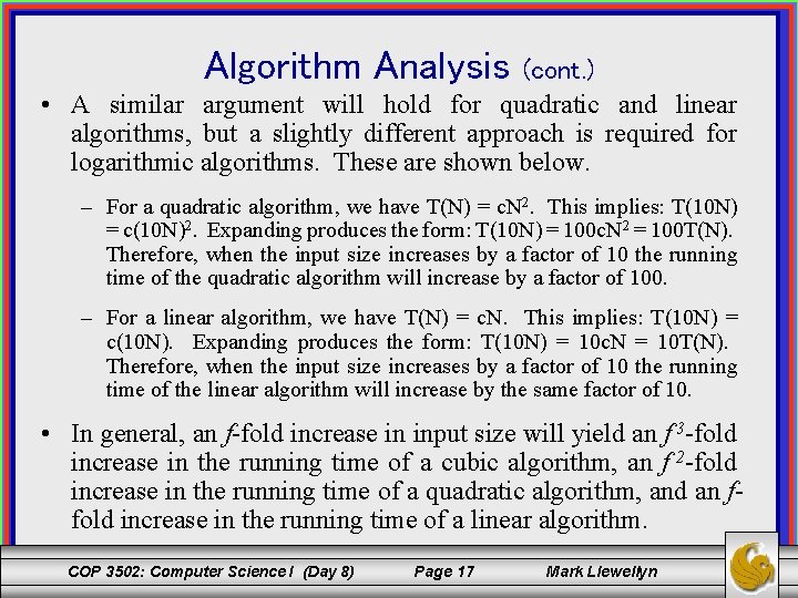
Algorithm Analysis (cont. ) • A similar argument will hold for quadratic and linear algorithms, but a slightly different approach is required for logarithmic algorithms. These are shown below. – For a quadratic algorithm, we have T(N) = c. N 2. This implies: T(10 N) = c(10 N)2. Expanding produces the form: T(10 N) = 100 c. N 2 = 100 T(N). Therefore, when the input size increases by a factor of 10 the running time of the quadratic algorithm will increase by a factor of 100. – For a linear algorithm, we have T(N) = c. N. This implies: T(10 N) = c(10 N). Expanding produces the form: T(10 N) = 10 c. N = 10 T(N). Therefore, when the input size increases by a factor of 10 the running time of the linear algorithm will increase by the same factor of 10. • In general, an f-fold increase in input size will yield an f 3 -fold increase in the running time of a cubic algorithm, an f 2 -fold increase in the running time of a quadratic algorithm, and an ffold increase in the running time of a linear algorithm. COP 3502: Computer Science I (Day 8) Page 17 Mark Llewellyn

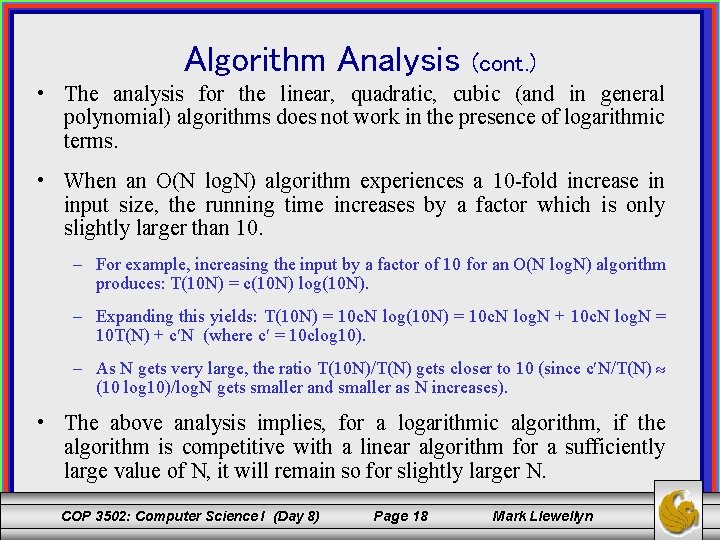
Algorithm Analysis (cont. ) • The analysis for the linear, quadratic, cubic (and in general polynomial) algorithms does not work in the presence of logarithmic terms. • When an O(N log. N) algorithm experiences a 10 -fold increase in input size, the running time increases by a factor which is only slightly larger than 10. – For example, increasing the input by a factor of 10 for an O(N log. N) algorithm produces: T(10 N) = c(10 N) log(10 N). – Expanding this yields: T(10 N) = 10 c. N log. N + 10 c. N log. N = 10 T(N) + c N (where c = 10 clog 10). – As N gets very large, the ratio T(10 N)/T(N) gets closer to 10 (since c N/T(N) (10 log 10)/log. N gets smaller and smaller as N increases). • The above analysis implies, for a logarithmic algorithm, if the algorithm is competitive with a linear algorithm for a sufficiently large value of N, it will remain so for slightly larger N. COP 3502: Computer Science I (Day 8) Page 18 Mark Llewellyn

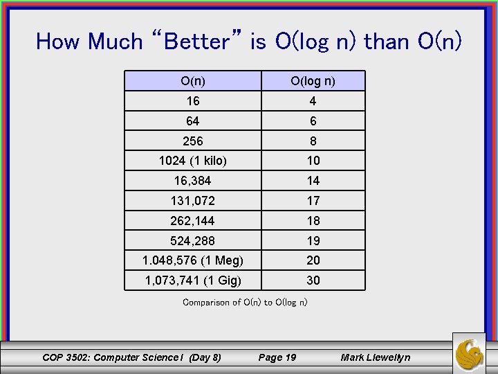
How Much “Better” is O(log n) than O(n) O(log n) 16 4 64 6 256 8 1024 (1 kilo) 10 16, 384 14 131, 072 17 262, 144 18 524, 288 19 1. 048, 576 (1 Meg) 20 1, 073, 741 (1 Gig) 30 Comparison of O(n) to O(log n) COP 3502: Computer Science I (Day 8) Page 19 Mark Llewellyn

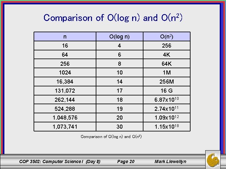
Comparison of O(log n) and O(n 2) n O(log n) O(n 2) 16 4 256 64 6 4 K 256 8 64 K 1024 10 1 M 16, 384 14 256 M 131, 072 17 16 G 262, 144 18 6. 87 x 1010 524, 288 19 2. 74 x 1011 1. 048, 576 20 1. 09 x 1012 1, 073, 741 30 1. 15 x 1018 Comparison of O(log n) and O(n 2) COP 3502: Computer Science I (Day 8) Page 20 Mark Llewellyn

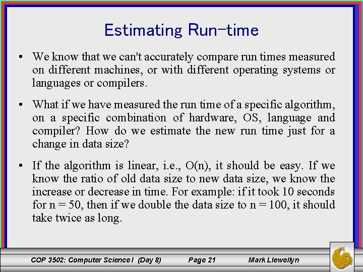
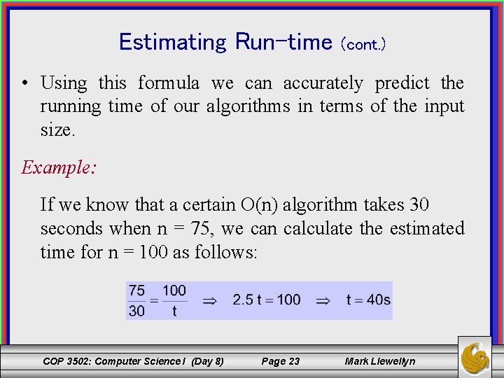
Estimating Run-time • We know that we can't accurately compare run times measured on different machines, or with different operating systems or languages or compilers. • What if we have measured the run time of a specific algorithm, on a specific combination of hardware, OS, language and compiler? How do we estimate the new run time just for a change in data size? • If the algorithm is linear, i. e. , O(n), it should be easy. If we know the ratio of old data size to new data size, we know the increase or decrease in time. For example: if it took 10 seconds for n = 50, then if we double the data size to n = 100, it should take twice as long. COP 3502: Computer Science I (Day 8) Page 21 Mark Llewellyn

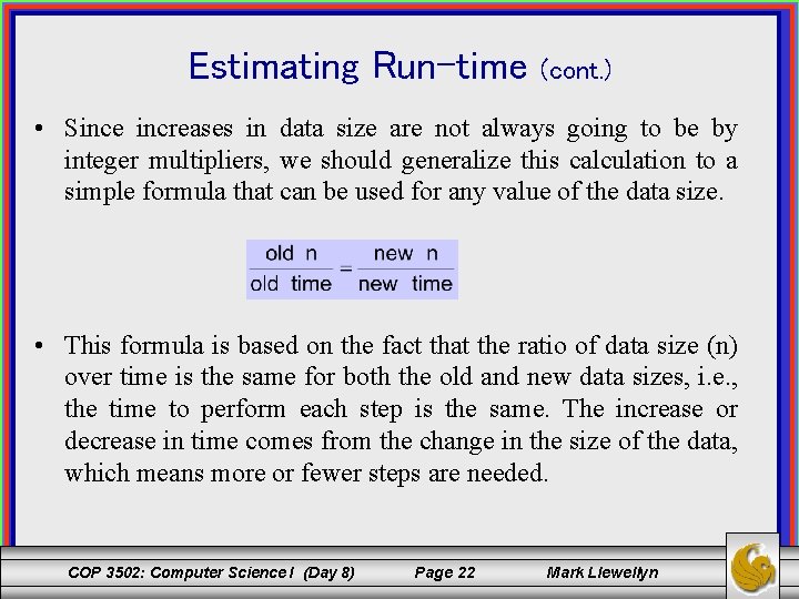
Estimating Run-time (cont. ) • Since increases in data size are not always going to be by integer multipliers, we should generalize this calculation to a simple formula that can be used for any value of the data size. • This formula is based on the fact that the ratio of data size (n) over time is the same for both the old and new data sizes, i. e. , the time to perform each step is the same. The increase or decrease in time comes from the change in the size of the data, which means more or fewer steps are needed. COP 3502: Computer Science I (Day 8) Page 22 Mark Llewellyn

Estimating Run-time (cont. ) • Using this formula we can accurately predict the running time of our algorithms in terms of the input size. Example: If we know that a certain O(n) algorithm takes 30 seconds when n = 75, we can calculate the estimated time for n = 100 as follows: COP 3502: Computer Science I (Day 8) Page 23 Mark Llewellyn

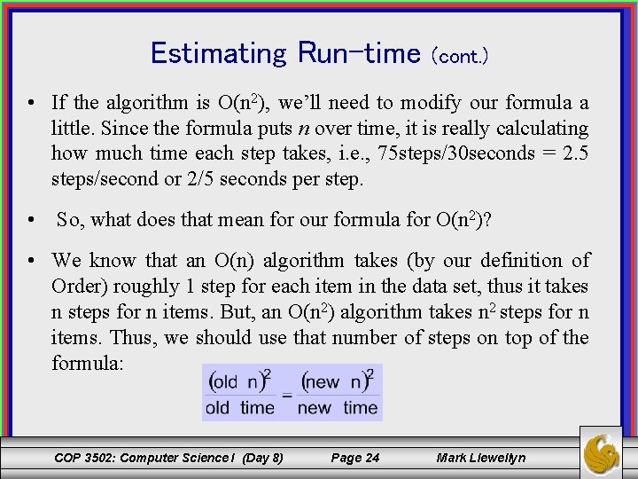
Estimating Run-time (cont. ) • If the algorithm is O(n 2), we’ll need to modify our formula a little. Since the formula puts n over time, it is really calculating how much time each step takes, i. e. , 75 steps/30 seconds = 2. 5 steps/second or 2/5 seconds per step. • So, what does that mean for our formula for O(n 2)? • We know that an O(n) algorithm takes (by our definition of Order) roughly 1 step for each item in the data set, thus it takes n steps for n items. But, an O(n 2) algorithm takes n 2 steps for n items. Thus, we should use that number of steps on top of the formula: COP 3502: Computer Science I (Day 8) Page 24 Mark Llewellyn

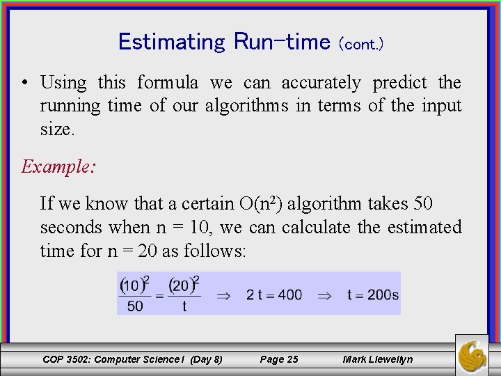
Estimating Run-time (cont. ) • Using this formula we can accurately predict the running time of our algorithms in terms of the input size. Example: If we know that a certain O(n 2) algorithm takes 50 seconds when n = 10, we can calculate the estimated time for n = 20 as follows: COP 3502: Computer Science I (Day 8) Page 25 Mark Llewellyn

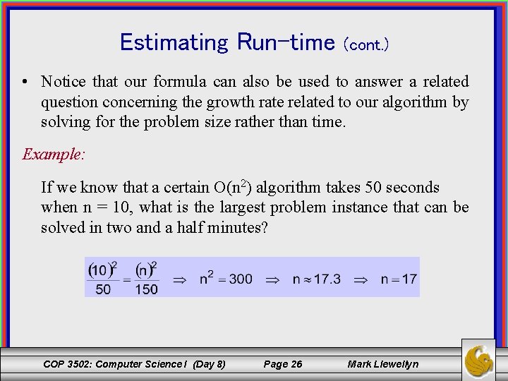
Estimating Run-time (cont. ) • Notice that our formula can also be used to answer a related question concerning the growth rate related to our algorithm by solving for the problem size rather than time. Example: If we know that a certain O(n 2) algorithm takes 50 seconds when n = 10, what is the largest problem instance that can be solved in two and a half minutes? COP 3502: Computer Science I (Day 8) Page 26 Mark Llewellyn

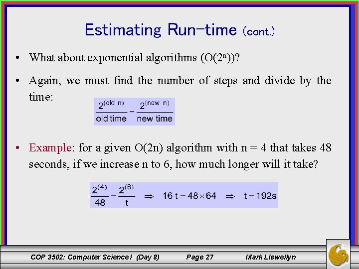
Estimating Run-time (cont. ) • What about exponential algorithms (O(2 n))? • Again, we must find the number of steps and divide by the time: • Example: for a given O(2 n) algorithm with n = 4 that takes 48 seconds, if we increase n to 6, how much longer will it take? COP 3502: Computer Science I (Day 8) Page 27 Mark Llewellyn

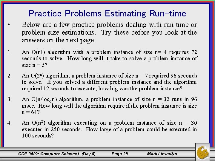
Practice Problems Estimating Run-time • Below are a few practice problems dealing with run-time or problem size estimations. Try these before you look at the answers on the next page. 1. An O(n!) algorithm with a problem instance of size n= 4 requires 72 seconds to solve. How long will it take to solve a problem instance of size n = 5? 2. An O(2 n) algorithm, a problem instance of size n = 7 required 96 seconds to solve. If you solved a different problem instance and the algorithm required 12 seconds to execute, how big was the problem instance? 3. An O(n/log 2 n) algorithm, a problem instance of size n = 32 runs in 96 msec. How long will the algorithm require if the problem instance is size n = 64? 4. An O(n 2) algorithm executing on a problem instance of size n = 30 executes in 250 seconds. How large of a problem could be executed in 100 seconds? COP 3502: Computer Science I (Day 8) Page 28 Mark Llewellyn

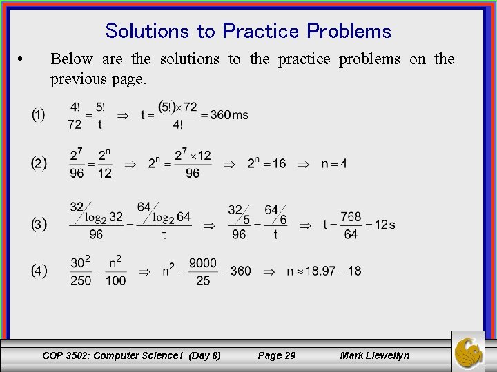
Solutions to Practice Problems • Below are the solutions to the practice problems on the previous page. COP 3502: Computer Science I (Day 8) Page 29 Mark Llewellyn