Computational Complexity Theory Lecture 5 Diagonalization Time Hierarchy







- Slides: 73
Computational Complexity Theory Lecture 5: Diagonalization, Time Hierarchy, Ladner’s theorem Indian Institute of Science
Recap: NTMs �A nondeterministic Turing machine is like a deterministic Turing machines but with two transition functions. �It is formally defined by a tuple (Γ, Q, δ 0 , δ 1). It has a special state qaccept in addition to qstart and qhalt. �At every step of computation, the machine applies one of two functions δ 0 and δ 1 arbitrarily. �Unlike DTMs, NTMs are not intended to be physically realizable (because of the arbitrary nature of application of the transition functions).
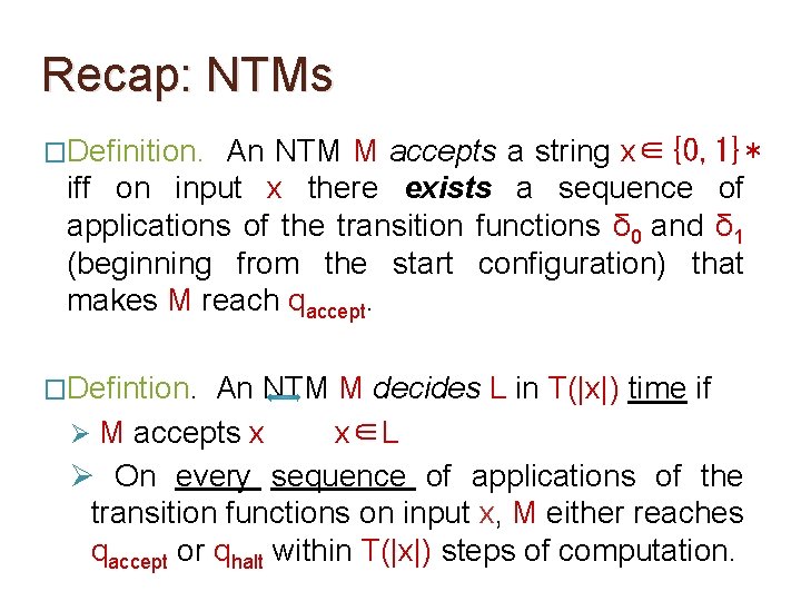
Recap: NTMs �Definition. An NTM M accepts a string x∈{0, 1}* iff on input x there exists a sequence of applications of the transition functions δ 0 and δ 1 (beginning from the start configuration) that makes M reach qaccept. �Defintion. An NTM M decides a language L ⊆ {0, 1}* if Ø M accepts x x∈L Ø On every sequence of applications of the transition functions on input x, M either reaches q or q.
Recap: NTMs �Definition. An NTM M accepts a string x∈{0, 1}* iff on input x there exists a sequence of applications of the transition functions δ 0 and δ 1 (beginning from the start configuration) that makes M reach qaccept. �Defintion. An NTM M decides L in T(|x|) time if Ø M accepts x x∈L Ø On every sequence of applications of the transition functions on input x, M either reaches qaccept or qhalt within T(|x|) steps of computation.
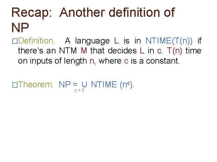
Recap: Another definition of NP �Definition. A language L is in NTIME(T(n)) if there’s an NTM M that decides L in c. T(n) time on inputs of length n, where c is a constant. �Theorem. NP = ∪ NTIME (nc). c>0
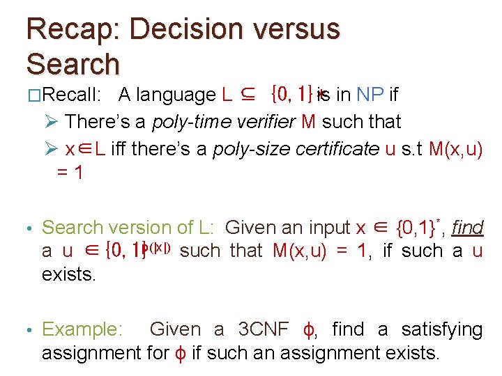
Recap: Decision versus Search �Recall: A language L ⊆ {0, 1}*is in NP if Ø There’s a poly-time verifier M such that Ø x∈L iff there’s a poly-size certificate u s. t M(x, u) =1 • Search version of L: Given an input x ∈ {0, 1}*, find a u ∈{0, 1}p(|x|) such that M(x, u) = 1, if such a u exists. • Example: Given a 3 CNF ϕ, find a satisfying assignment for ϕ if such an assignment exists.
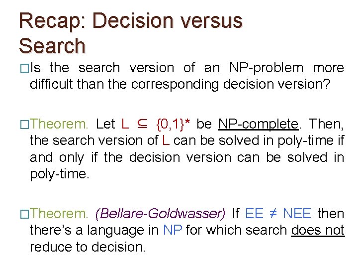
Recap: Decision versus Search �Is the search version of an NP-problem more difficult than the corresponding decision version? �Theorem. Let L ⊆ {0, 1}* be NP-complete. Then, the search version of L can be solved in poly-time if and only if the decision version can be solved in poly-time. �Theorem. (Bellare-Goldwasser) If EE ≠ NEE then there’s a language in NP for which search does not reduce to decision.
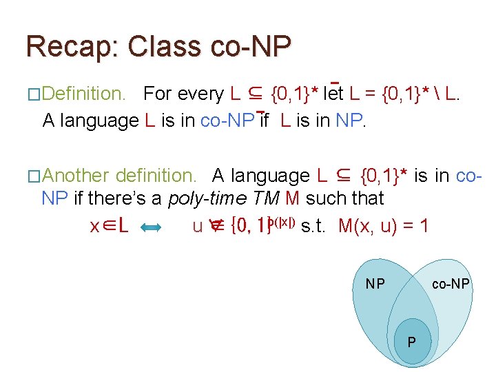
Recap: Class co-NP �Definition. For every L ⊆ {0, 1}* let L = {0, 1}* L. A language L is in co-NP if L is in NP. �Another definition. A language L ⊆ {0, 1}* is in co. NP if there’s a poly-time TM M such that x∈L u∀ ∈{0, 1}p(|x|) s. t. M(x, u) = 1 NP co-NP P
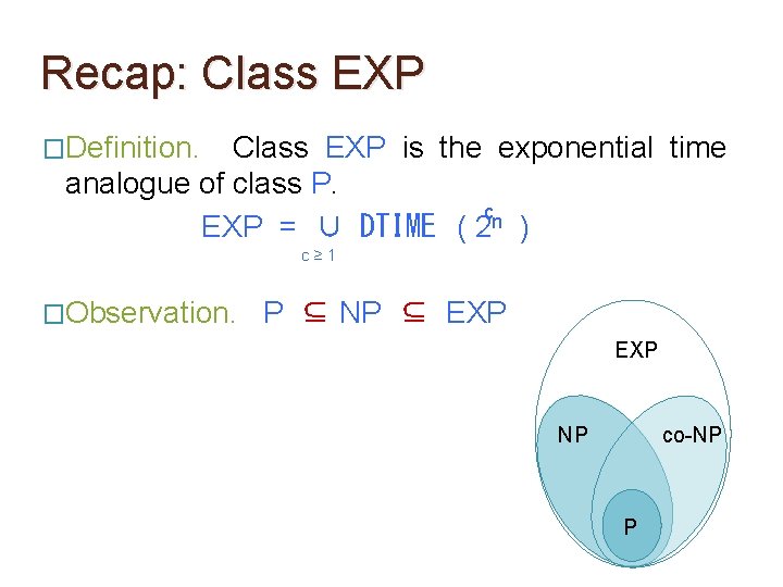
Recap: Class EXP �Definition. Class EXP is the exponential time analogue of class P. cn EXP = ∪ DTIME ( 2 ) c≥ 1 �Observation. P ⊆ NP ⊆ EXP NP co-NP P
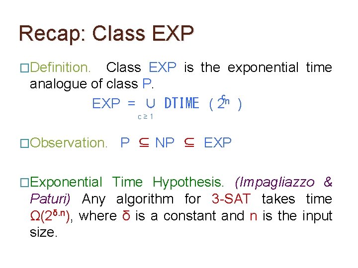
Recap: Class EXP �Definition. Class EXP is the exponential time analogue of class P. cn EXP = ∪ DTIME ( 2 ) c≥ 1 �Observation. �Exponential P ⊆ NP ⊆ EXP Time Hypothesis. (Impagliazzo & Paturi) Any algorithm for 3 -SAT takes time Ω(2δ. n), where δ is a constant and n is the input size.
Diagonalization
Diagonalization �Diagonalization refers to a class of techniques used in complexity theory to separate complexity classes.
Diagonalization �Diagonalization refers to a class of techniques used in complexity theory to separate complexity classes. �These techniques are characterized by two main features:
Diagonalization �Diagonalization refers to a class of techniques used in complexity theory to separate complexity classes. �These techniques are characterized by two main features: 1. There’s a universal TM U that when given strings α and x, simulates Mα on x with only a small overhead.
Diagonalization �Diagonalization refers to a class of techniques used in complexity theory to separate complexity classes. �These techniques are characterized by two main features: 1. There’s a universal TM U that when given strings α and x, simulates Mα on x with only a small overhead. If Mα takes T time on x then U takes O(T log T) time to simulate Mα on x.
Diagonalization �Diagonalization refers to a class of techniques used in complexity theory to separate complexity classes. �These techniques are characterized by two main features: 1. There’s a universal TM U that when given strings α and x, simulates Mα on x with only a small overhead. 2. Every string represents some TM, and every TM can be represented by infinitely many strings.
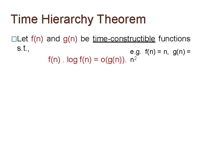
Time Hierarchy Theorem �Let s. t. , f(n) and g(n) be time-constructible functions e. g. f(n) = n, g(n) = f(n). log f(n) = o(g(n)). n 2
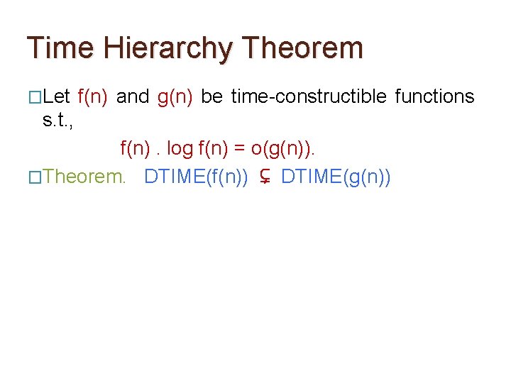
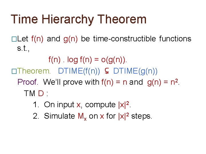
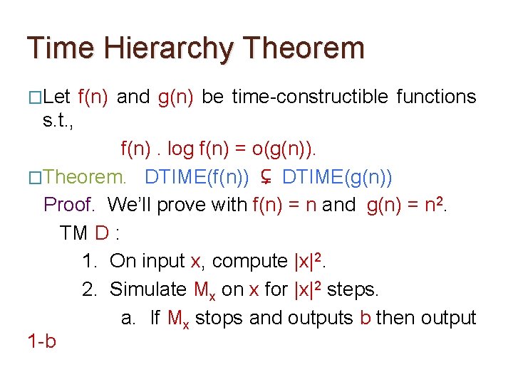
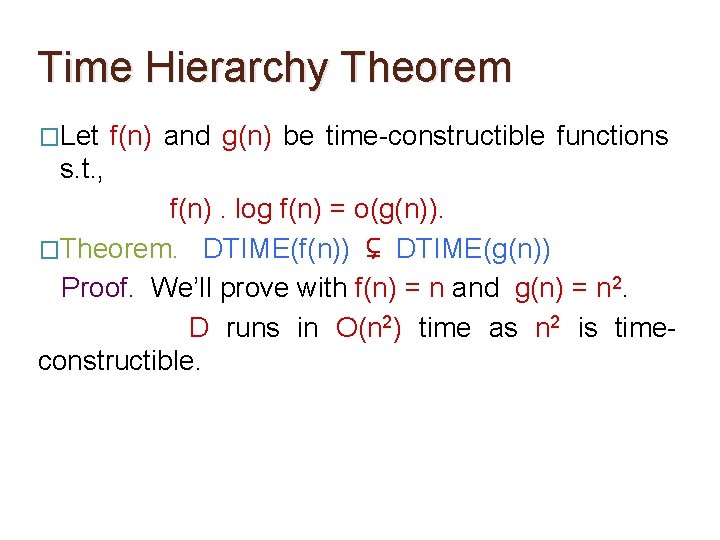
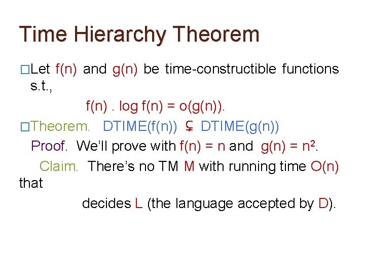
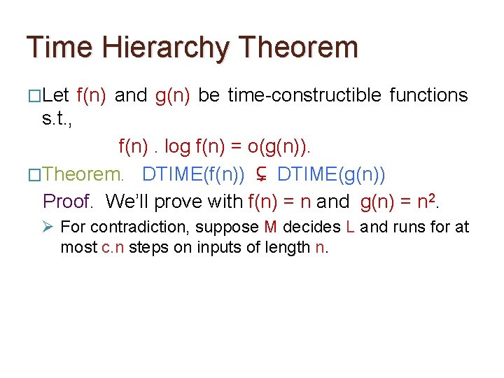
Time Hierarchy Theorem �Let f(n) and g(n) be time-constructible functions s. t. , f(n). log f(n) = o(g(n)). �Theorem. DTIME(f(n)) ⊊ DTIME(g(n))
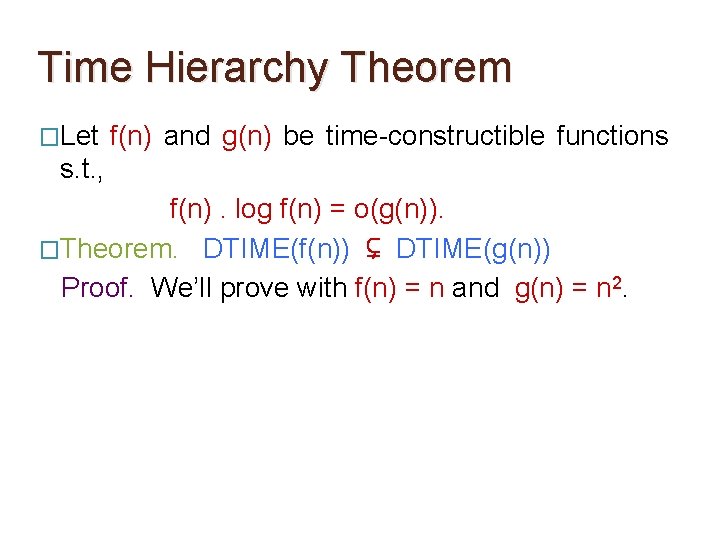
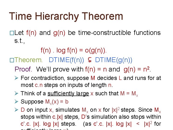
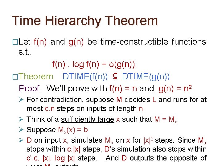
Time Hierarchy Theorem �Let f(n) and g(n) be time-constructible functions s. t. , f(n). log f(n) = o(g(n)). �Theorem. DTIME(f(n)) ⊊ DTIME(g(n)) Proof. We’ll prove with f(n) = n and g(n) = n 2.
Time Hierarchy Theorem �Let f(n) and g(n) be time-constructible functions s. t. , f(n). log f(n) = o(g(n)). �Theorem. DTIME(f(n)) ⊊ DTIME(g(n)) Proof. We’ll prove with f(n) = n and g(n) = n 2. Task: Show that there’s a language L decided by a TM D with time complexity O(n 2) s. t. , any TM M with runtime O(n) cannot decide L.
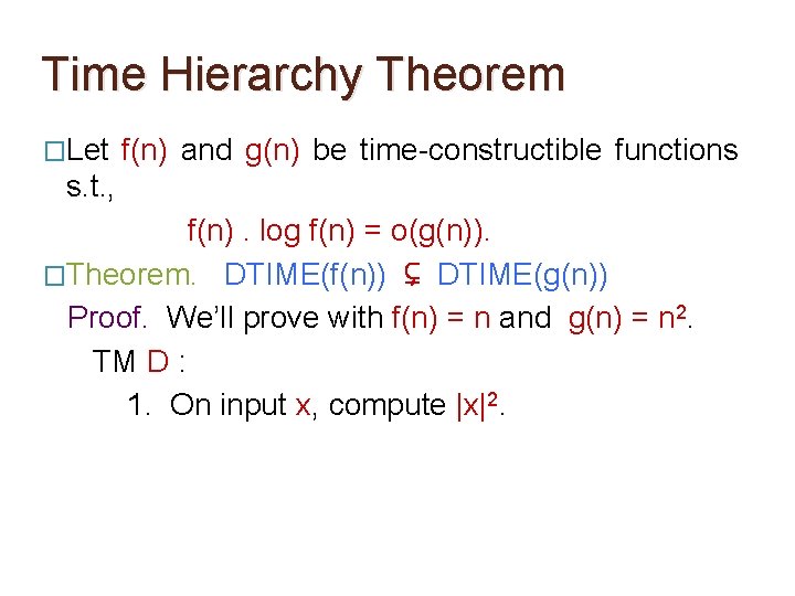
Time Hierarchy Theorem �Let f(n) and g(n) be time-constructible functions s. t. , f(n). log f(n) = o(g(n)). �Theorem. DTIME(f(n)) ⊊ DTIME(g(n)) Proof. We’ll prove with f(n) = n and g(n) = n 2. TM D : 1. On input x, compute |x|2.
Time Hierarchy Theorem �Let f(n) and g(n) be time-constructible functions s. t. , f(n). log f(n) = o(g(n)). �Theorem. DTIME(f(n)) ⊊ DTIME(g(n)) Proof. We’ll prove with f(n) = n and g(n) = n 2. TM D : 1. On input x, compute |x|2. 2. Simulate Mx on x for |x|2 steps.
Time Hierarchy Theorem �Let f(n) and g(n) be time-constructible functions s. t. , f(n). log f(n) = o(g(n)). �Theorem. DTIME(f(n)) ⊊ DTIME(g(n)) Proof. We’ll prove with f(n) = n and g(n) = n 2. TM D : 1. On input x, compute |x|2. 2. Simulate Mx on x for |x|2 steps. a. If Mx stops and outputs b then output 1 -b
Time Hierarchy Theorem �Let f(n) and g(n) be time-constructible functions s. t. , f(n). log f(n) = o(g(n)). �Theorem. DTIME(f(n)) ⊊ DTIME(g(n)) Proof. We’ll prove with f(n) = n and g(n) = n 2. TM D : 1. On input x, compute |x|2. 2. Simulate Mx on x for |x|2 steps. a. If Mx stops and outputs b then output 1 -b b. otherwise, output 1.
Time Hierarchy Theorem �Let f(n) and g(n) be time-constructible functions s. t. , f(n). log f(n) = o(g(n)). �Theorem. DTIME(f(n)) ⊊ DTIME(g(n)) Proof. We’ll prove with f(n) = n and g(n) = n 2. D runs in O(n 2) time as n 2 is timeconstructible.
Time Hierarchy Theorem �Let f(n) and g(n) be time-constructible functions s. t. , f(n). log f(n) = o(g(n)). �Theorem. DTIME(f(n)) ⊊ DTIME(g(n)) Proof. We’ll prove with f(n) = n and g(n) = n 2. Claim. There’s no TM M with running time O(n) that decides L (the language accepted by D).
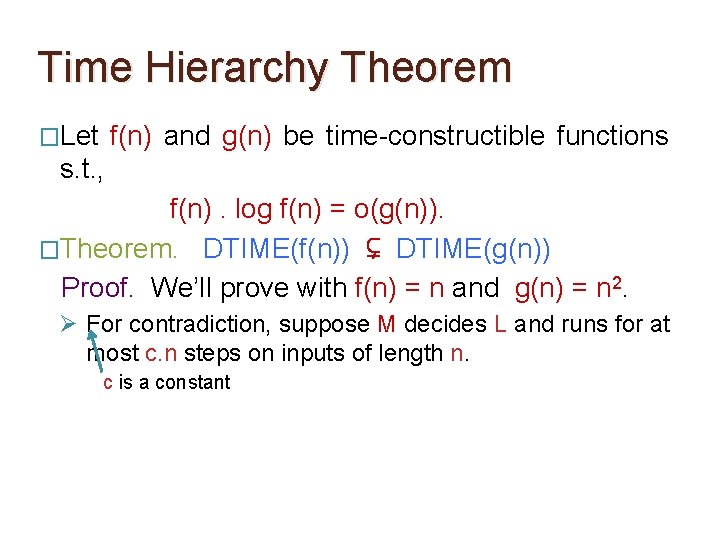
Time Hierarchy Theorem �Let f(n) and g(n) be time-constructible functions s. t. , f(n). log f(n) = o(g(n)). �Theorem. DTIME(f(n)) ⊊ DTIME(g(n)) Proof. We’ll prove with f(n) = n and g(n) = n 2. Ø For contradiction, suppose M decides L and runs for at most c. n steps on inputs of length n.
Time Hierarchy Theorem �Let f(n) and g(n) be time-constructible functions s. t. , f(n). log f(n) = o(g(n)). �Theorem. DTIME(f(n)) ⊊ DTIME(g(n)) Proof. We’ll prove with f(n) = n and g(n) = n 2. Ø For contradiction, suppose M decides L and runs for at most c. n steps on inputs of length n. c is a constant
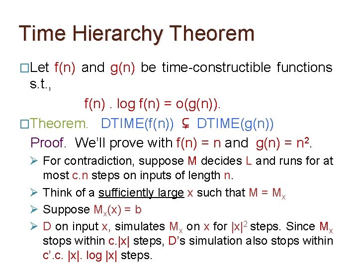
Time Hierarchy Theorem �Let f(n) and g(n) be time-constructible functions s. t. , f(n). log f(n) = o(g(n)). �Theorem. DTIME(f(n)) ⊊ DTIME(g(n)) Proof. We’ll prove with f(n) = n and g(n) = n 2. Ø For contradiction, suppose M decides L and runs for at most c. n steps on inputs of length n. Ø Think of a sufficiently large x such that M = Mx
Time Hierarchy Theorem �Let f(n) and g(n) be time-constructible functions s. t. , f(n). log f(n) = o(g(n)). �Theorem. DTIME(f(n)) ⊊ DTIME(g(n)) Proof. We’ll prove with f(n) = n and g(n) = n 2. Ø For contradiction, suppose M decides L and runs for at most c. n steps on inputs of length n. Ø Think of a sufficiently large x such that M = Mx Ø Suppose Mx(x) = b
Time Hierarchy Theorem �Let f(n) and g(n) be time-constructible functions s. t. , f(n). log f(n) = o(g(n)). �Theorem. DTIME(f(n)) ⊊ DTIME(g(n)) Proof. We’ll prove with f(n) = n and g(n) = n 2. Ø For contradiction, suppose M decides L and runs for at most c. n steps on inputs of length n. Ø Think of a sufficiently large x such that M = Mx Ø Suppose Mx(x) = b Ø D on input x, simulates Mx on x for |x|2 steps.
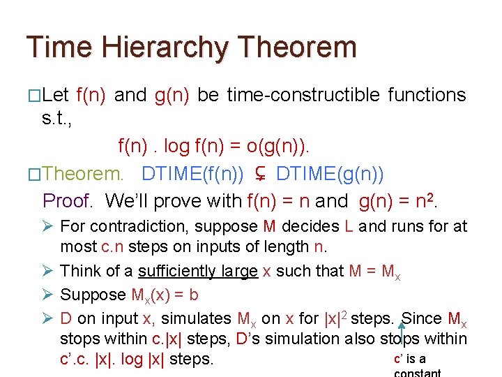
Time Hierarchy Theorem �Let f(n) and g(n) be time-constructible functions s. t. , f(n). log f(n) = o(g(n)). �Theorem. DTIME(f(n)) ⊊ DTIME(g(n)) Proof. We’ll prove with f(n) = n and g(n) = n 2. Ø For contradiction, suppose M decides L and runs for at most c. n steps on inputs of length n. Ø Think of a sufficiently large x such that M = Mx Ø Suppose Mx(x) = b Ø D on input x, simulates Mx on x for |x|2 steps. Since Mx stops within c. |x| steps, D’s simulation also stops within c’. c. |x|. log |x| steps.
Time Hierarchy Theorem �Let f(n) and g(n) be time-constructible functions s. t. , f(n). log f(n) = o(g(n)). �Theorem. DTIME(f(n)) ⊊ DTIME(g(n)) Proof. We’ll prove with f(n) = n and g(n) = n 2. Ø For contradiction, suppose M decides L and runs for at most c. n steps on inputs of length n. Ø Think of a sufficiently large x such that M = Mx Ø Suppose Mx(x) = b Ø D on input x, simulates Mx on x for |x|2 steps. Since Mx stops within c. |x| steps, D’s simulation also stops within c’ is a c’. c. |x|. log |x| steps.
Time Hierarchy Theorem �Let f(n) and g(n) be time-constructible functions s. t. , f(n). log f(n) = o(g(n)). �Theorem. DTIME(f(n)) ⊊ DTIME(g(n)) Proof. We’ll prove with f(n) = n and g(n) = n 2. Ø For contradiction, suppose M decides L and runs for at most c. n steps on inputs of length n. Ø Think of a sufficiently large x such that M = Mx Ø Suppose Mx(x) = b Ø D on input x, simulates Mx on x for |x|2 steps. Since Mx stops within c. |x| steps, D’s simulation also stops within c’. c. |x|. log |x| steps. (as c’. c. |x|. log |x| < |x|2 for
Time Hierarchy Theorem �Let f(n) and g(n) be time-constructible functions s. t. , f(n). log f(n) = o(g(n)). �Theorem. DTIME(f(n)) ⊊ DTIME(g(n)) Proof. We’ll prove with f(n) = n and g(n) = n 2. Ø For contradiction, suppose M decides L and runs for at most c. n steps on inputs of length n. Ø Think of a sufficiently large x such that M = Mx Ø Suppose Mx(x) = b Ø D on input x, simulates Mx on x for |x|2 steps. Since Mx stops within c. |x| steps, D’s simulation also stops within c’. c. |x|. log |x| steps. And D outputs the opposite of
Time Hierarchy Theorem �Let f(n) and g(n) be time-constructible functions s. t. , f(n). log f(n) = o(g(n)). �Theorem. DTIME(f(n)) ⊊ DTIME(g(n)) Proof. We’ll prove with f(n) = n and g(n) = n 2. Ø For contradiction, suppose M decides L and runs for at most c. n steps on inputs of length n. Ø Think of a sufficiently large x such that M = Mx Ø Suppose Mx(x) = b Ø Hence, D(x) = 1 -b
Time Hierarchy Theorem �Let f(n) and g(n) be time-constructible functions s. t. , f(n). log f(n) = o(g(n)). �Theorem. DTIME(f(n)) ⊊ DTIME(g(n)) Proof. We’ll prove with f(n) = n and g(n) = n 2. Ø For contradiction, suppose M decides L and runs for at most c. n steps on inputs of length n. Ø Think of a sufficiently large x such that M = Mx Ø Suppose Mx(x) = b Ø Hence, D(x) = 1 -b Contradiction! M does not decide L.
Time Hierarchy Theorem �Let f(n) and g(n) be time-constructible functions s. t. , f(n). log f(n) = o(g(n)). �Theorem. DTIME(f(n)) ⊊ DTIME(g(n)) P ⊊ EXP
Time Hierarchy Theorem �Let f(n) and g(n) be time-constructible functions s. t. , f(n). log f(n) = o(g(n)). �Theorem. DTIME(f(n)) ⊊ DTIME(g(n)) P ⊊ EXP Proof. Similar (homework)
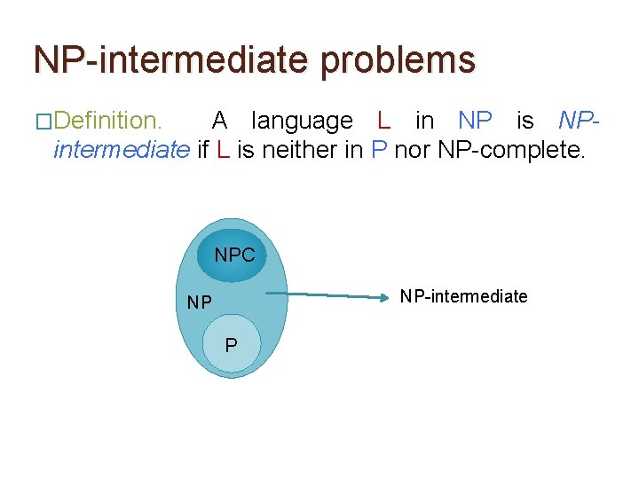
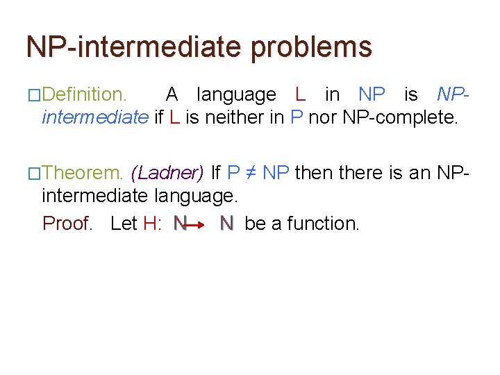
NP-intermediate problems �Definition. A language L in NP is NPintermediate if L is neither in P nor NP-complete.
NP-intermediate problems �Definition. A language L in NP is NPintermediate if L is neither in P nor NP-complete. NPC NP-intermediate NP P
NP-intermediate problems �Definition. A language L in NP is NPintermediate if L is neither in P nor NP-complete. … the notion makes sense only if P ≠ NP
NP-intermediate problems �Definition. A language L in NP is NPintermediate if L is neither in P nor NP-complete. �Theorem. (Ladner) If P ≠ NP then there is an NPintermediate language.
NP-intermediate problems �Definition. A language L in NP is NPintermediate if L is neither in P nor NP-complete. �Theorem. (Ladner) If P ≠ NP then there is an NPintermediate language. Proof. A delicate argument using diagonalization.
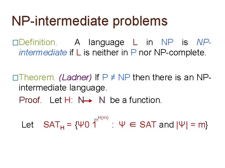
NP-intermediate problems �Definition. A language L in NP is NPintermediate if L is neither in P nor NP-complete. �Theorem. (Ladner) If P ≠ NP then there is an NPintermediate language. Proof. Let H: N N be a function.
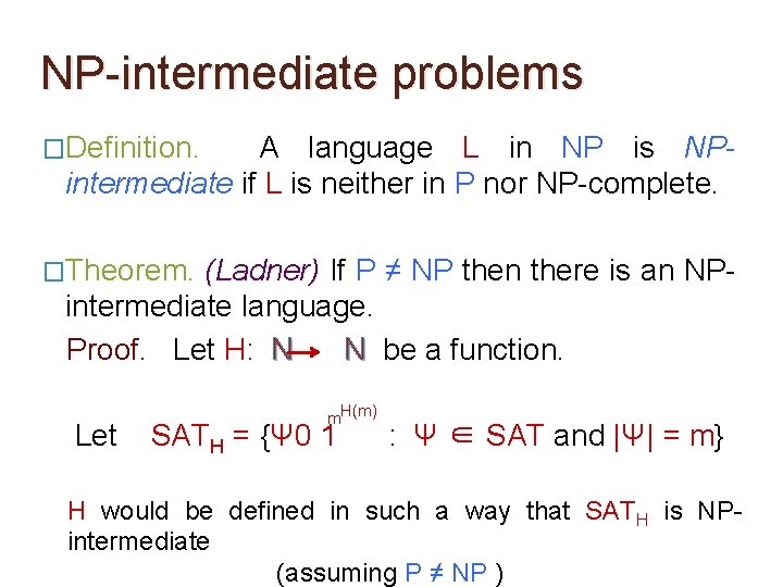
NP-intermediate problems �Definition. A language L in NP is NPintermediate if L is neither in P nor NP-complete. �Theorem. (Ladner) If P ≠ NP then there is an NPintermediate language. Proof. Let H: N N be a function. Let m. H(m) SATH = {Ψ 0 1 : Ψ ∈ SAT and |Ψ| = m}
NP-intermediate problems �Definition. A language L in NP is NPintermediate if L is neither in P nor NP-complete. �Theorem. (Ladner) If P ≠ NP then there is an NPintermediate language. Proof. Let H: N N be a function. Let m. H(m) SATH = {Ψ 0 1 : Ψ ∈ SAT and |Ψ| = m} H would be defined in such a way that SATH is NPintermediate (assuming P ≠ NP )
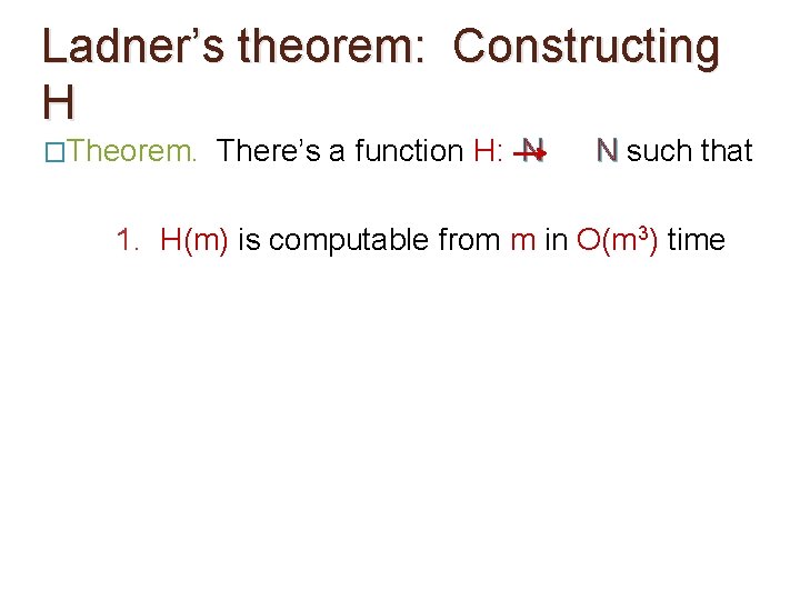
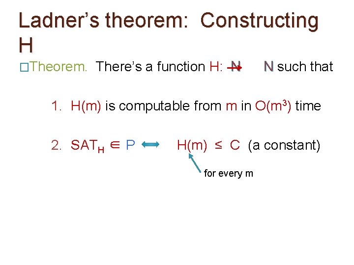
Ladner’s theorem: Constructing H �Theorem. There’s a function H: N N such that 1. H(m) is computable from m in O(m 3) time
Ladner’s theorem: Constructing H �Theorem. There’s a function H: N N such that 1. H(m) is computable from m in O(m 3) time 2. SATH ∈ P H(m) ≤ C (a constant) for every m
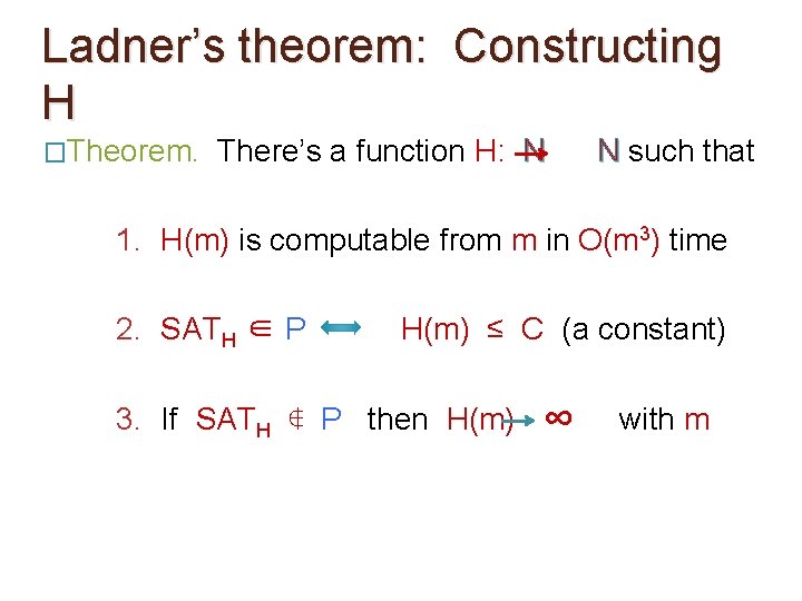
Ladner’s theorem: Constructing H �Theorem. There’s a function H: N N such that 1. H(m) is computable from m in O(m 3) time 2. SATH ∈ P H(m) ≤ C (a constant) 3. If SATH ∉ P then H(m) ∞ with m
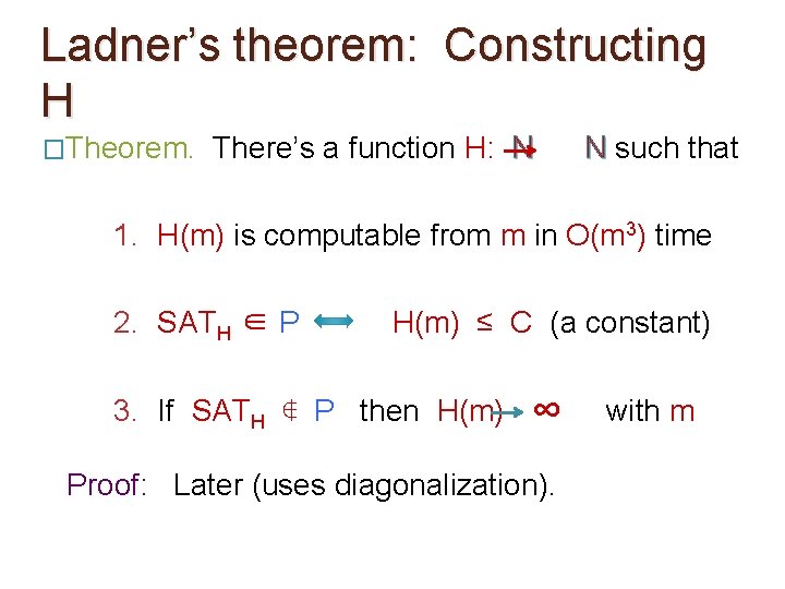
Ladner’s theorem: Constructing H �Theorem. There’s a function H: N N such that 1. H(m) is computable from m in O(m 3) time 2. SATH ∈ P H(m) ≤ C (a constant) 3. If SATH ∉ P then H(m) ∞ Proof: Later (uses diagonalization). with m
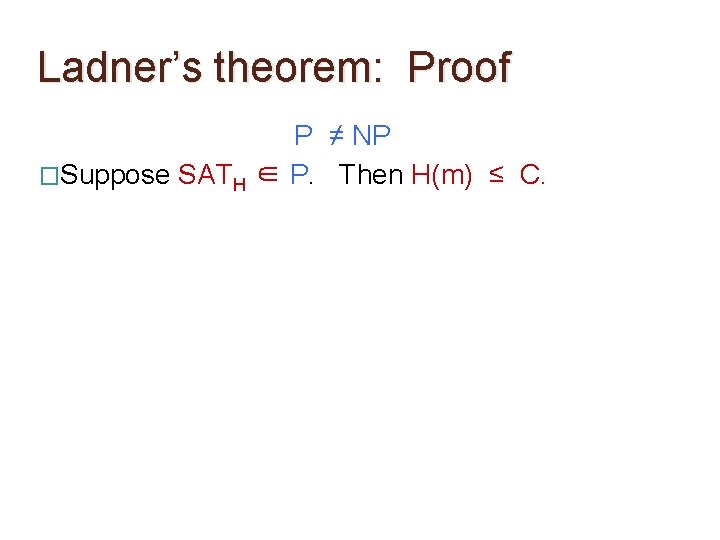
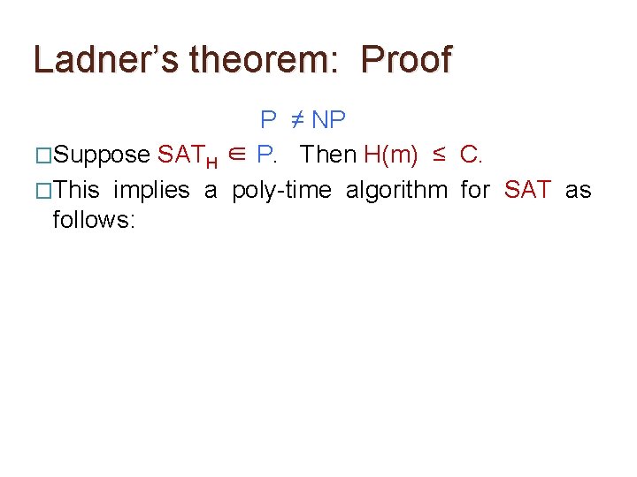
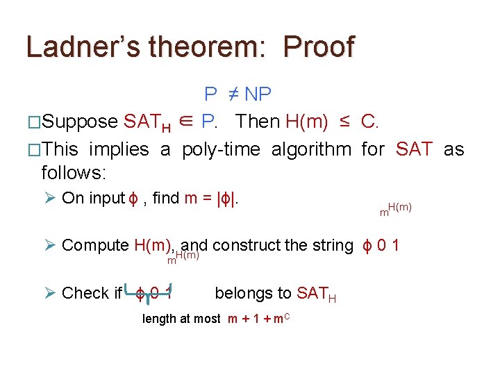
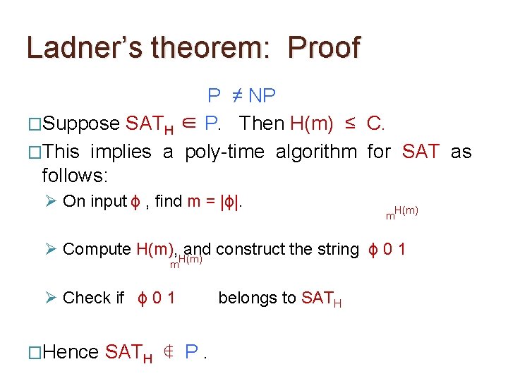
Ladner’s theorem: Proof P ≠ NP �Suppose SATH ∈ P. Then H(m) ≤ C.
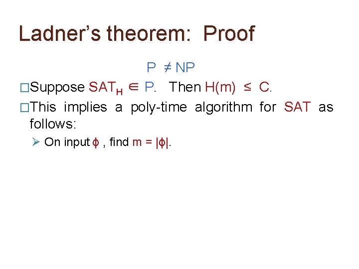
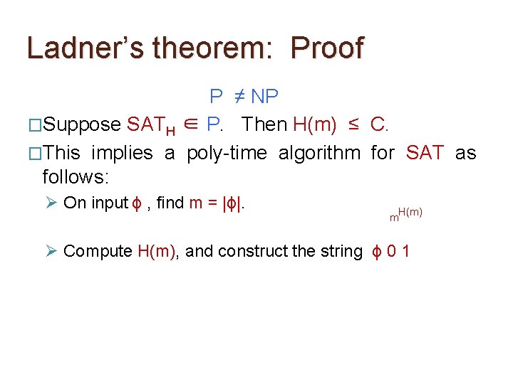
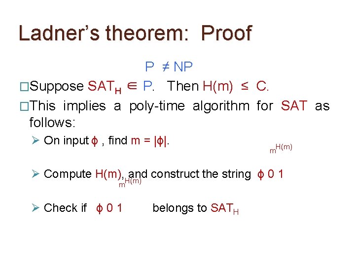
Ladner’s theorem: Proof P ≠ NP �Suppose SATH ∈ P. Then H(m) ≤ C. �This implies a poly-time algorithm for SAT as follows:
Ladner’s theorem: Proof P ≠ NP �Suppose SATH ∈ P. Then H(m) ≤ C. �This implies a poly-time algorithm for SAT as follows: Ø On input ϕ , find m = |ϕ|.
Ladner’s theorem: Proof P ≠ NP �Suppose SATH ∈ P. Then H(m) ≤ C. �This implies a poly-time algorithm for SAT as follows: Ø On input ϕ , find m = |ϕ|. m. H(m) Ø Compute H(m), and construct the string ϕ 0 1
Ladner’s theorem: Proof P ≠ NP �Suppose SATH ∈ P. Then H(m) ≤ C. �This implies a poly-time algorithm for SAT as follows: Ø On input ϕ , find m = |ϕ|. m. H(m) Ø Compute H(m), H(m) and construct the string ϕ 0 1 m Ø Check if ϕ 0 1 belongs to SATH
Ladner’s theorem: Proof P ≠ NP �Suppose SATH ∈ P. Then H(m) ≤ C. �This implies a poly-time algorithm for SAT as follows: Ø On input ϕ , find m = |ϕ|. m. H(m) Ø Compute H(m), H(m) and construct the string ϕ 0 1 m Ø Check if ϕ 0 1 belongs to SATH length at most m + 1 + m. C
Ladner’s theorem: Proof P ≠ NP �Suppose SATH ∈ P. Then H(m) ≤ C. �This implies a poly-time algorithm for SAT as follows: Ø On input ϕ , find m = |ϕ|. m. H(m) Ø Compute H(m), H(m) and construct the string ϕ 0 1 m Ø Check if ϕ 0 1 �Hence SATH ∉ P. belongs to SATH
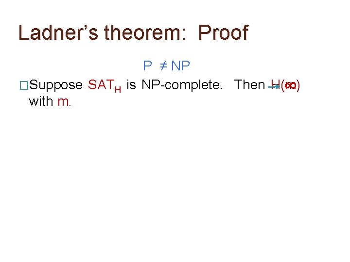
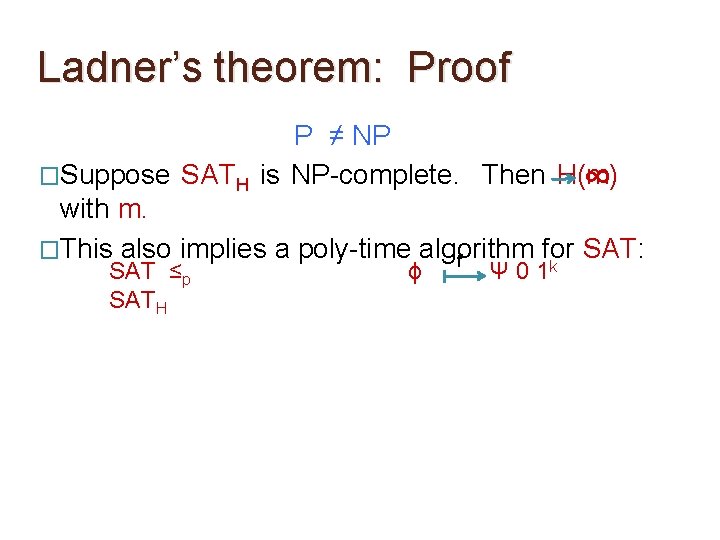
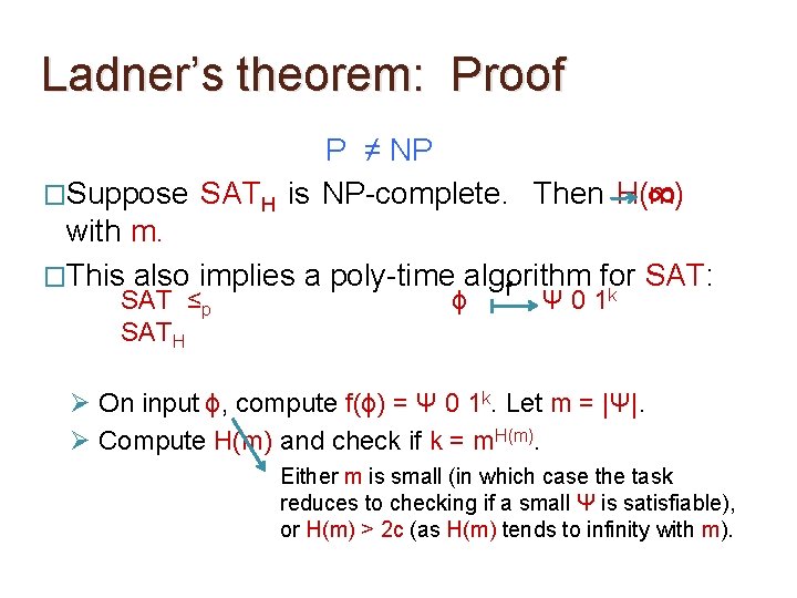
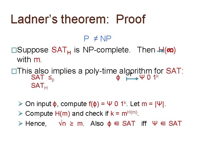
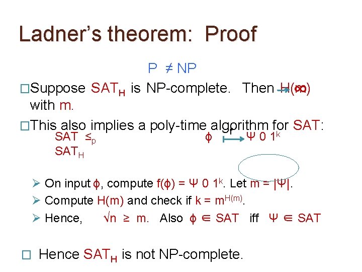
Ladner’s theorem: Proof P ≠ NP �Suppose SATH is NP-complete. Then H(m) ∞ with m.
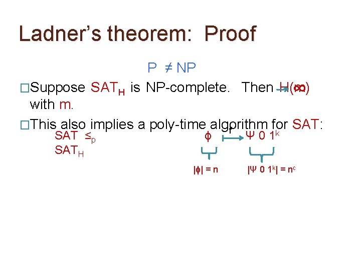
Ladner’s theorem: Proof P ≠ NP �Suppose SATH is NP-complete. Then H(m) ∞ with m. �This also implies a poly-time algorithm for SAT: f SAT ≤p SATH ϕ Ψ 0 1 k
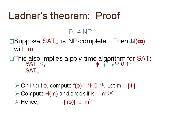
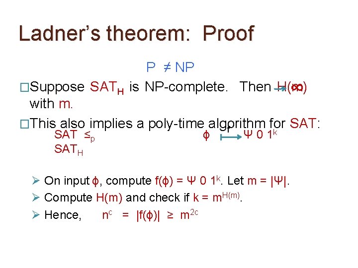
Ladner’s theorem: Proof P ≠ NP �Suppose SATH is NP-complete. Then H(m) ∞ with m. �This also implies a poly-time algorithm for SAT: f SAT ≤p SATH ϕ |ϕ| = n Ψ 0 1 k |Ψ 0 1 k| = nc
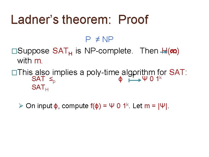
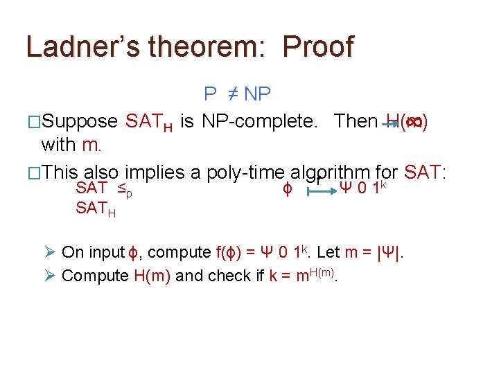
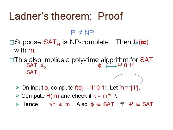
Ladner’s theorem: Proof P ≠ NP �Suppose SATH is NP-complete. Then H(m) ∞ with m. �This also implies a poly-time algorithm for SAT: f SAT ≤p SATH ϕ Ψ 0 1 k Ø On input ϕ, compute f(ϕ) = Ψ 0 1 k. Let m = |Ψ|.
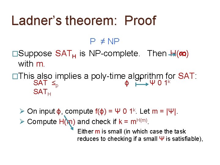
Ladner’s theorem: Proof P ≠ NP �Suppose SATH is NP-complete. Then H(m) ∞ with m. �This also implies a poly-time algorithm for SAT: f SAT ≤p SATH ϕ Ψ 0 1 k Ø On input ϕ, compute f(ϕ) = Ψ 0 1 k. Let m = |Ψ|. Ø Compute H(m) and check if k = m. H(m).
Ladner’s theorem: Proof P ≠ NP �Suppose SATH is NP-complete. Then H(m) ∞ with m. �This also implies a poly-time algorithm for SAT: f SAT ≤p SATH ϕ Ψ 0 1 k Ø On input ϕ, compute f(ϕ) = Ψ 0 1 k. Let m = |Ψ|. Ø Compute H(m) and check if k = m. H(m). Either m is small (in which case the task reduces to checking if a small Ψ is satisfiable),
Ladner’s theorem: Proof P ≠ NP �Suppose SATH is NP-complete. Then H(m) ∞ with m. �This also implies a poly-time algorithm for SAT: f SAT ≤p SATH ϕ Ψ 0 1 k Ø On input ϕ, compute f(ϕ) = Ψ 0 1 k. Let m = |Ψ|. Ø Compute H(m) and check if k = m. H(m). Either m is small (in which case the task reduces to checking if a small Ψ is satisfiable), or H(m) > 2 c (as H(m) tends to infinity with m).
Ladner’s theorem: Proof P ≠ NP �Suppose SATH is NP-complete. Then H(m) ∞ with m. �This also implies a poly-time algorithm for SAT: f SAT ≤p SATH ϕ Ψ 0 1 k Ø On input ϕ, compute f(ϕ) = Ψ 0 1 k. Let m = |Ψ|. Ø Compute H(m) and check if k = m. H(m). Ø Hence, |f(ϕ)| ≥ m 2 c
Ladner’s theorem: Proof P ≠ NP �Suppose SATH is NP-complete. Then H(m) ∞ with m. �This also implies a poly-time algorithm for SAT: f SAT ≤p SATH ϕ Ψ 0 1 k Ø On input ϕ, compute f(ϕ) = Ψ 0 1 k. Let m = |Ψ|. Ø Compute H(m) and check if k = m. H(m). Ø Hence, nc = |f(ϕ)| ≥ m 2 c
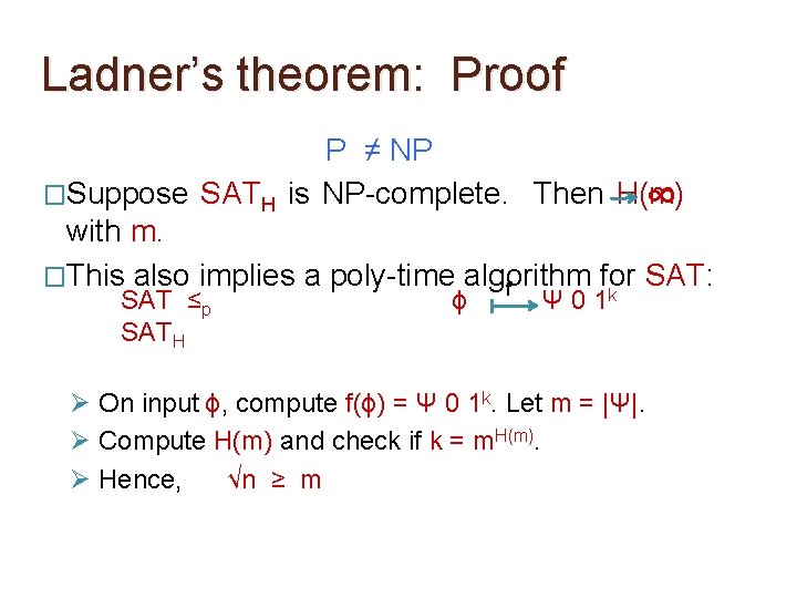
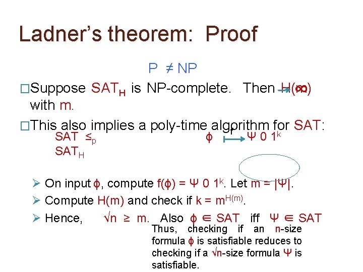
Ladner’s theorem: Proof P ≠ NP �Suppose SATH is NP-complete. Then H(m) ∞ with m. �This also implies a poly-time algorithm for SAT: f SAT ≤p SATH ϕ Ψ 0 1 k Ø On input ϕ, compute f(ϕ) = Ψ 0 1 k. Let m = |Ψ|. Ø Compute H(m) and check if k = m. H(m). Ø Hence, √n ≥ m
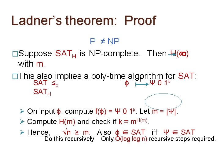
Ladner’s theorem: Proof P ≠ NP �Suppose SATH is NP-complete. Then H(m) ∞ with m. �This also implies a poly-time algorithm for SAT: f SAT ≤p SATH ϕ Ψ 0 1 k Ø On input ϕ, compute f(ϕ) = Ψ 0 1 k. Let m = |Ψ|. Ø Compute H(m) and check if k = m. H(m). Ø Hence, √n ≥ m. Also ϕ ∈ SAT iff Ψ ∈ SAT
Ladner’s theorem: Proof P ≠ NP �Suppose SATH is NP-complete. Then H(m) ∞ with m. �This also implies a poly-time algorithm for SAT: f SAT ≤p SATH ϕ Ψ 0 1 k Ø On input ϕ, compute f(ϕ) = Ψ 0 1 k. Let m = |Ψ|. Ø Compute H(m) and check if k = m. H(m). Ø Hence, √n ≥ m. Also ϕ ∈ SAT iff Ψ ∈ SAT
Ladner’s theorem: Proof P ≠ NP �Suppose SATH is NP-complete. Then H(m) ∞ with m. �This also implies a poly-time algorithm for SAT: f SAT ≤p SATH ϕ Ψ 0 1 k Ø On input ϕ, compute f(ϕ) = Ψ 0 1 k. Let m = |Ψ|. Ø Compute H(m) and check if k = m. H(m). Ø Hence, √n ≥ m. Also ϕ ∈ SAT iff Ψ ∈ SAT Thus, checking if an n-size formula ϕ is satisfiable reduces to checking if a √n-size formula Ψ is satisfiable.
Ladner’s theorem: Proof P ≠ NP �Suppose SATH is NP-complete. Then H(m) ∞ with m. �This also implies a poly-time algorithm for SAT: f SAT ≤p SATH ϕ Ψ 0 1 k Ø On input ϕ, compute f(ϕ) = Ψ 0 1 k. Let m = |Ψ|. Ø Compute H(m) and check if k = m. H(m). Ø Hence, √n ≥ m. Also ϕ ∈ SAT iff Ψ ∈ SAT Do this recursively! Only O(log n) recursive steps required.
Ladner’s theorem: Proof P ≠ NP �Suppose SATH is NP-complete. Then H(m) ∞ with m. �This also implies a poly-time algorithm for SAT: f SAT ≤p SATH ϕ Ψ 0 1 k Ø On input ϕ, compute f(ϕ) = Ψ 0 1 k. Let m = |Ψ|. Ø Compute H(m) and check if k = m. H(m). Ø Hence, √n ≥ m. Also ϕ ∈ SAT iff Ψ ∈ SAT � Hence SATH is not NP-complete.