Complexity and Performance Binary Search Average case Assume

Complexity and Performance

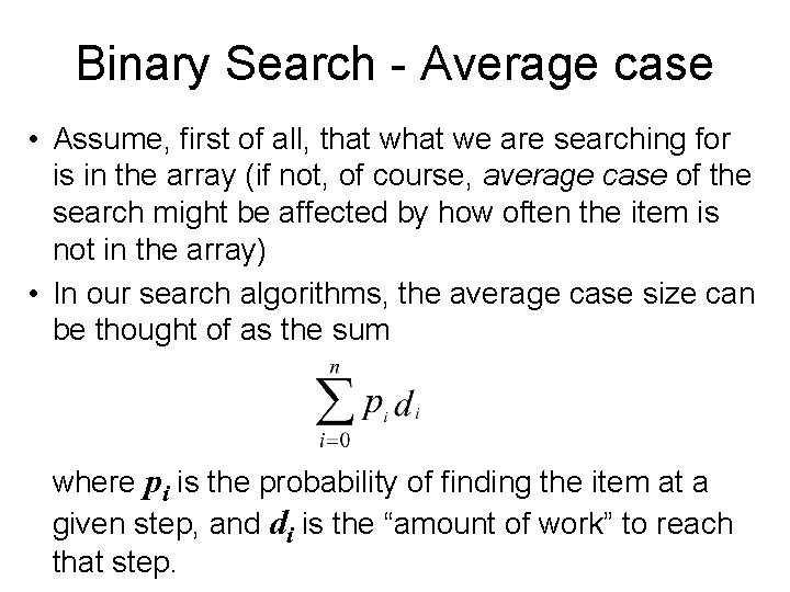
Binary Search - Average case • Assume, first of all, that we are searching for is in the array (if not, of course, average case of the search might be affected by how often the item is not in the array) • In our search algorithms, the average case size can be thought of as the sum where pi is the probability of finding the item at a given step, and di is the “amount of work” to reach that step.

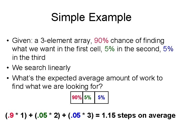
Simple Example • Given: a 3 -element array, 90% chance of finding what we want in the first cell, 5% in the second, 5% in the third • We search linearly • What’s the expected average amount of work to find what we are looking for? 90% 5% 5% (. 9 * 1) + (. 05 * 2) + (. 05 * 3) = 1. 15 steps on average

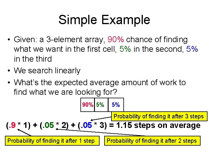
Simple Example • Given: a 3 -element array, 90% chance of finding what we want in the first cell, 5% in the second, 5% in the third • We search linearly • What’s the expected average amount of work to find what we are looking for? 90% 5% 5% Probability of finding it after 3 steps (. 9 * 1) + (. 05 * 2) + (. 05 * 3) = 1. 15 steps on average Probability of finding it after 1 step Probability of finding it after 2 steps

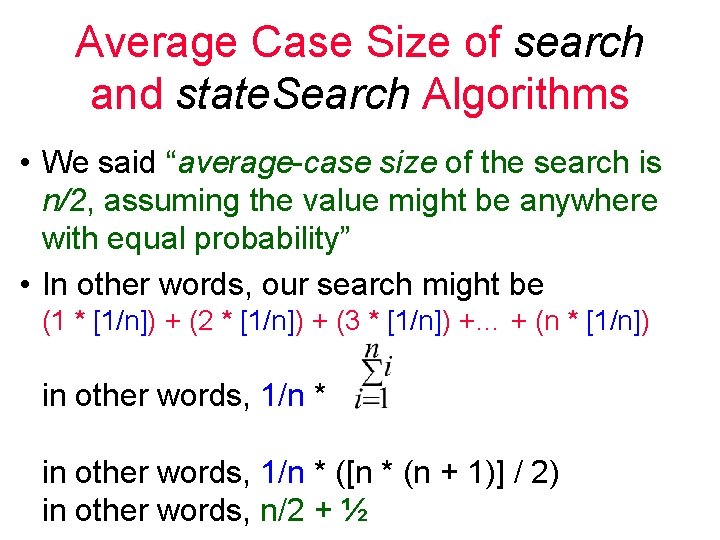
Average Case Size of search and state. Search Algorithms • We said “average-case size of the search is n/2, assuming the value might be anywhere with equal probability” • In other words, our search might be (1 * [1/n]) + (2 * [1/n]) + (3 * [1/n]) +… + (n * [1/n]) in other words, 1/n * ([n * (n + 1)] / 2) in other words, n/2 + ½

Constants Fade in Importance • We will see soon that if the expected amount of work is: n/2 + ½ what really interests us is the “shape” of the function • The ½ fades away for large n • Even the division of n by 2 is basically unimportant (since we didn’t really quantify how much work each cell of the array took) • What’s important is that the expected work grows linearly with the size of the array (i. e. , the input)

Asymptotic Behavior of (Some) Functions

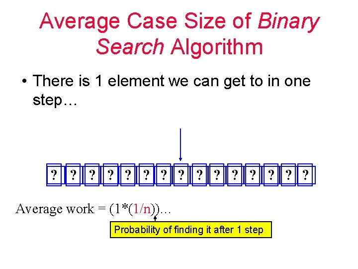
Average Case Size of Binary Search Algorithm • There is 1 element we can get to in one step… ? ? ? ? Average work = (1*(1/n))… Probability of finding it after 1 step

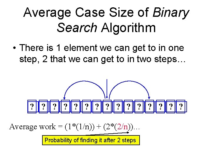
Average Case Size of Binary Search Algorithm • There is 1 element we can get to in one step, 2 that we can get to in two steps… ? ? ? ? Average work = (1*(1/n)) + (2*(2/n))… Probability of finding it after 2 steps

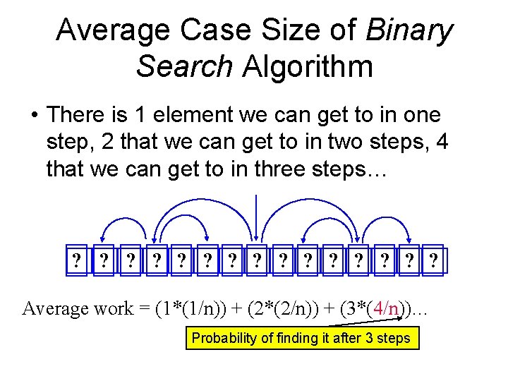
Average Case Size of Binary Search Algorithm • There is 1 element we can get to in one step, 2 that we can get to in two steps, 4 that we can get to in three steps… ? ? ? ? Average work = (1*(1/n)) + (2*(2/n)) + (3*(4/n))… Probability of finding it after 3 steps

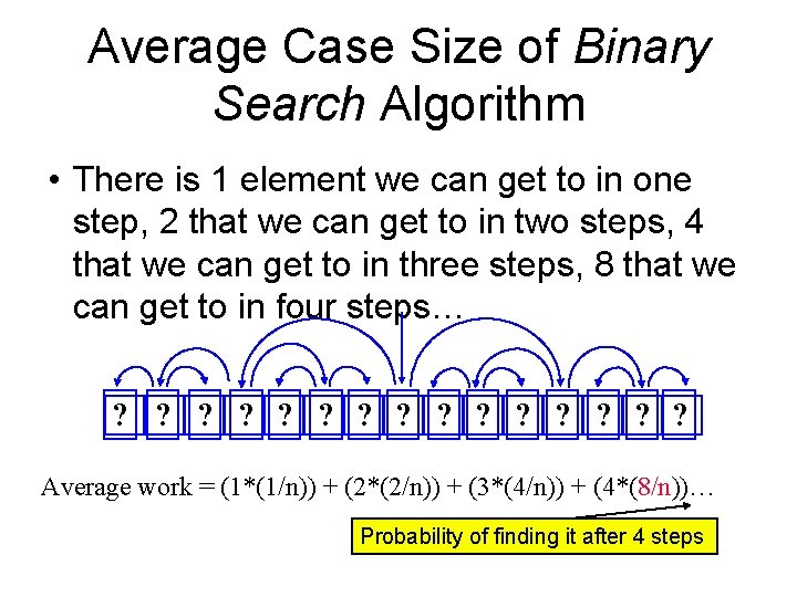
Average Case Size of Binary Search Algorithm • There is 1 element we can get to in one step, 2 that we can get to in two steps, 4 that we can get to in three steps, 8 that we can get to in four steps… ? ? ? ? Average work = (1*(1/n)) + (2*(2/n)) + (3*(4/n)) + (4*(8/n))… Probability of finding it after 4 steps

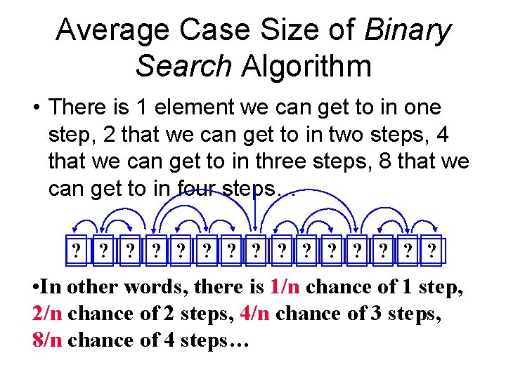
Average Case Size of Binary Search Algorithm • There is 1 element we can get to in one step, 2 that we can get to in two steps, 4 that we can get to in three steps, 8 that we can get to in four steps… ? ? ? ? • In other words, there is 1/n chance of 1 step, 2/n chance of 2 steps, 4/n chance of 3 steps, 8/n chance of 4 steps…

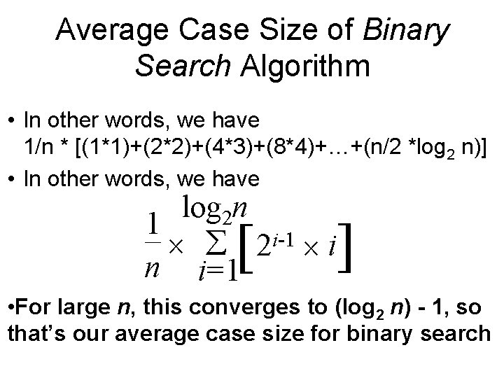
Average Case Size of Binary Search Algorithm • In other words, we have 1/n * [(1*1)+(2*2)+(4*3)+(8*4)+…+(n/2 *log 2 n)] • In other words, we have log 2 n 1 ´ å 2 i-1 ´ i n i=1 [ ] • For large n, this converges to (log 2 n) - 1, so that’s our average case size for binary search

Again, Constants Fade in Importance • If we calculated that the average case for binary search is (log 2 n) – 1 • We don’t care how much work we did in each cell • What’s really interesting is the “shape” of the function for large inputs (i. e. , large n) • So we would say that the average case for binary search is O(log 2 n) – read “Big-O” of log 2 n • We’ll define this precisely soon

Complexity and Performance • Some algorithms are better than others for solving the same problem • We can’t just measure run-time, because the number will vary depending on – what language was used to implement the algorithm, how well the program was written – how fast the computer is – how good the compiler is – how fast the hard disk was…

Basic idea: counting operations • Each algorithm performs a sequence of basic operations: – Arithmetic: (low + high)/2 – Comparison: if ( x > 0 ) … – Assignment: temp = x – Looping: while ( true ) { … } –… • Idea: count the number of basic operations performed on the input

It Depends • Difficulties: –Which operations are basic? –Not all operations take the same amount of time –Operations take different times with different hardware or compilers

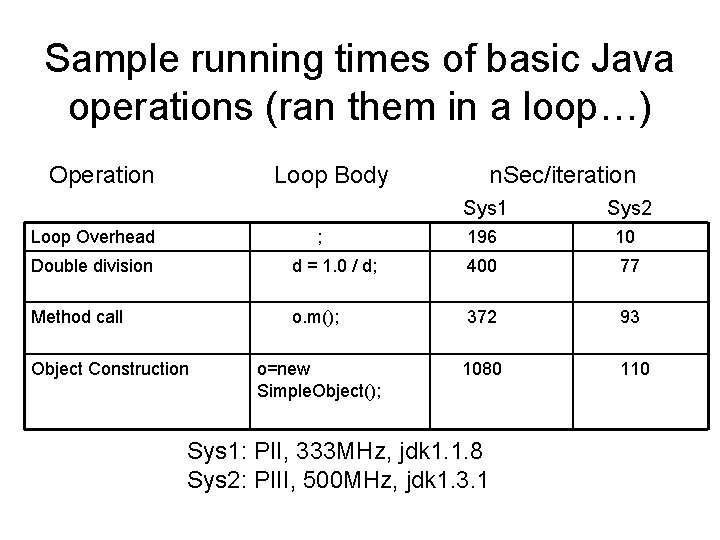
Sample running times of basic Java operations (ran them in a loop…) Operation Loop Body Loop Overhead ; n. Sec/iteration Sys 1 Sys 2 196 10 Double division d = 1. 0 / d; 400 77 Method call o. m(); 372 93 o=new Simple. Object(); 1080 110 Object Construction Sys 1: PII, 333 MHz, jdk 1. 1. 8 Sys 2: PIII, 500 MHz, jdk 1. 3. 1

So instead… • We use mathematical functions that estimate or bound: – the growth rate of a problem’s difficulty, or – the performance of an algorithm • Our Motivation: analyze the running time of an algorithm as a function of only simple parameters of the input

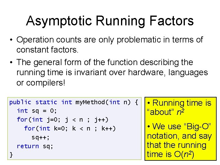
Asymptotic Running Factors • Operation counts are only problematic in terms of constant factors. • The general form of the function describing the running time is invariant over hardware, languages or compilers! public static int my. Method(int n) { int sq = 0; for(int j=0; j < n ; j++) for(int k=0; k < n ; k++) sq++; return sq; } • Running time is “about” n 2 • We use “Big-O” notation, and say that the running time is O(n 2)

The Problem’s Size • The problem’s size is stated in terms of n, which might be: – the number of components in an array – the number of items in a file – the number of pixels on a screen – the amount of output the program is expected to produce

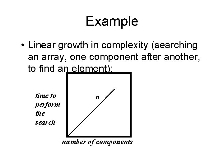
Example • Linear growth in complexity (searching an array, one component after another, to find an element): time to perform the search n number of components

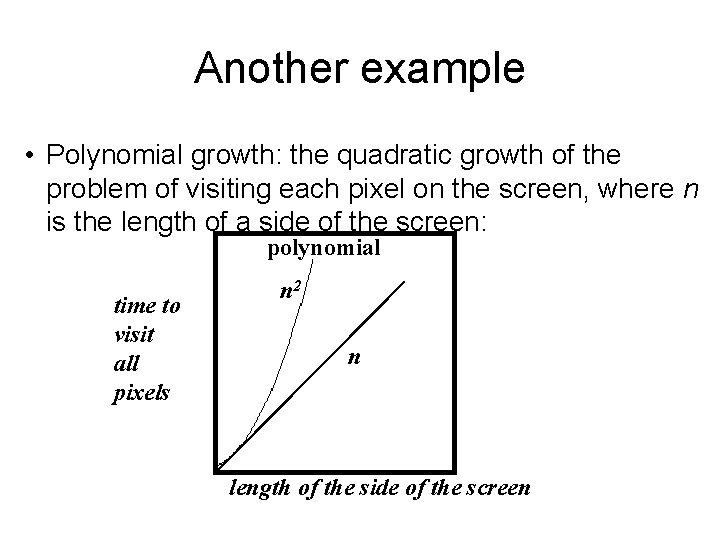
Another example • Polynomial growth: the quadratic growth of the problem of visiting each pixel on the screen, where n is the length of a side of the screen: polynomial time to visit all pixels n 2 n length of the side of the screen

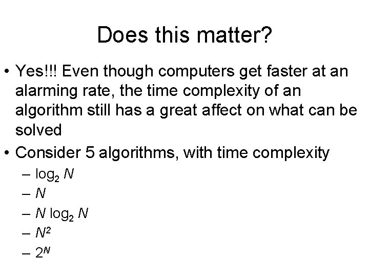
Does this matter? • Yes!!! Even though computers get faster at an alarming rate, the time complexity of an algorithm still has a great affect on what can be solved • Consider 5 algorithms, with time complexity – – – log 2 N N N log 2 N N 2 2 N

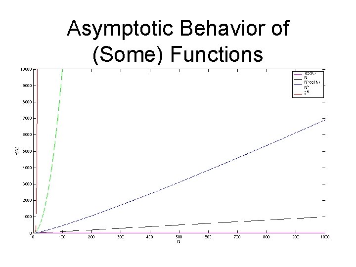
Asymptotic Behavior of (Some) Functions

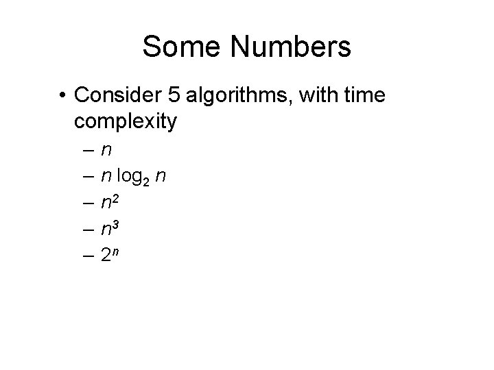
Some Numbers • Consider 5 algorithms, with time complexity – – – n n log 2 n n 2 n 3 2 n

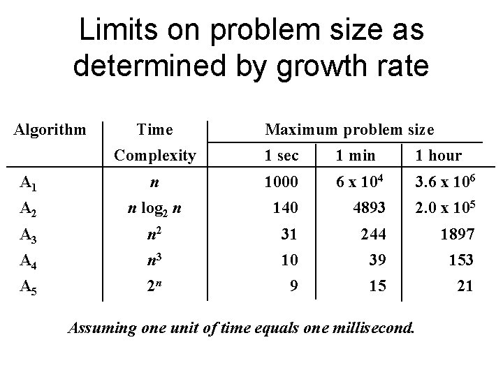
Limits on problem size as determined by growth rate Algorithm Time Maximum problem size Complexity 1 sec 1 min 1 hour A 1 n 1000 6 x 104 3. 6 x 106 A 2 n log 2 n 140 4893 2. 0 x 105 A 3 n 2 31 244 1897 A 4 n 3 10 39 153 A 5 2 n 9 15 21 Assuming one unit of time equals one millisecond.

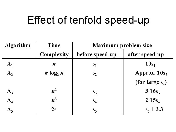
Effect of tenfold speed-up Algorithm Time Maximum problem size Complexity before speed-up after speed-up A 1 n s 1 10 s 1 A 2 n log 2 n s 2 Approx. 10 s 2 (for large s 2) A 3 n 2 s 3 3. 16 s 3 A 4 n 3 s 4 2. 15 s 4 A 5 2 n s 5 + 3. 3

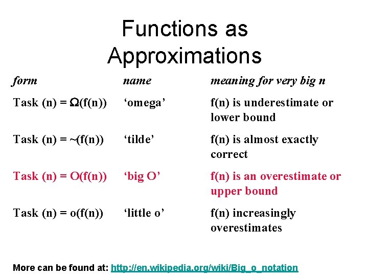
Functions as Approximations form name meaning for very big n Task (n) = (f(n)) ‘omega’ f(n) is underestimate or lower bound Task (n) = ~(f(n)) ‘tilde’ f(n) is almost exactly correct Task (n) = O(f(n)) ‘big O’ f(n) is an overestimate or upper bound Task (n) = o(f(n)) ‘little o’ f(n) increasingly overestimates More can be found at: http: //en. wikipedia. org/wiki/Big_o_notation

Big O Notation • Big O notation is the most useful for us; it says that a function f(n) serves as an upper bound on real-life performance. • For algorithm A of size n (informally): The complexity of A(n) is on the order of f(n) if A(n) is less than or equal to some constant times f(n) • The constant can be anything as long as the relation holds once n reaches some threshold.

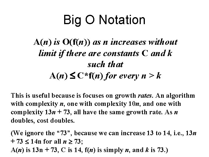
Big O Notation A(n) is O(f(n)) as n increases without limit if there are constants C and k such that A(n) C*f(n) for every n > k This is useful because is focuses on growth rates. An algorithm with complexity n, one with complexity 10 n, and one with complexity 13 n + 73, all have the same growth rate. As n doubles, cost doubles. (We ignore the “ 73”, because we can increase 13 to 14, i. e. , 13 n + 73 14 n for all n 73; A(n) is 13 n + 73, C is 14, f(n) is simply n, and k is 73. )

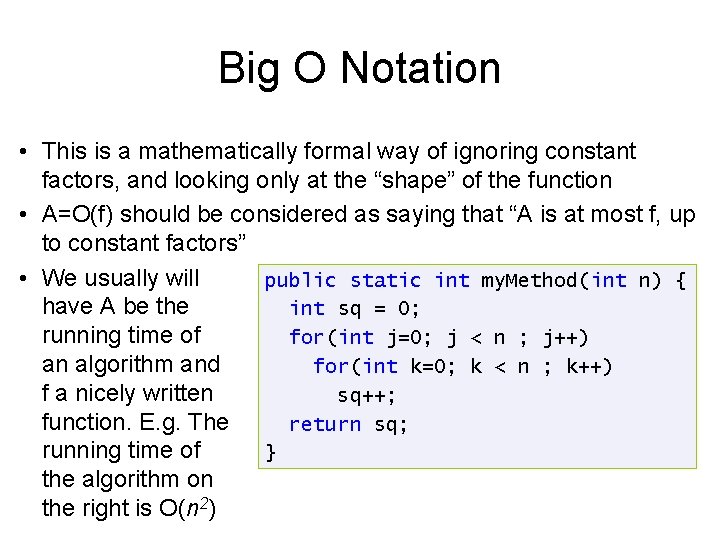
Big O Notation • This is a mathematically formal way of ignoring constant factors, and looking only at the “shape” of the function • A=O(f) should be considered as saying that “A is at most f, up to constant factors” • We usually will public static int my. Method(int n) { have A be the int sq = 0; running time of for(int j=0; j < n ; j++) an algorithm and for(int k=0; k < n ; k++) f a nicely written sq++; function. E. g. The return sq; running time of } the algorithm on the right is O(n 2)

Asymptotic Analysis of Algorithms • We usually embark on an asymptotic worst case analysis of the running time of the algorithm. • Asymptotic: – Formal, exact, depends only on the algorithm – Ignores constants – Applicable mostly for large input sizes • Worst Case: – Bounds on running time must hold for all inputs – Thus the analysis considers the worst-case input – Sometimes the “average” performance can be much better – Real-life inputs rarely “average” in any formal sense

Worst Case/Best Case • Worst case performance measure of an algorithm states an upper bound • Best case complexity measure of a problem states a lower bound; no algorithm can take less time

Multiplicative Factors • Because of multiplicative factors, it’s not always clear that an algorithm with a slower growth rate is better • If the real time complexities were A 1 = 1000 n, A 2 = 100 nlog 2 n, A 3 = 10 n 2, A 4 = n 3, and A 5 = 2 n, then A 5 is best for problems with n between 2 and 9, A 3 is best for problems with n between 10 and 58, A 2 is best for n between 59 and 1024, and A 1 is best for bigger n.

An Example: Binary Search • Binary search splits the unknown portion of the array in half; the worstcase search will be O(log 2 n) • Doubling n only increases the logarithm by 1; growth is very slow

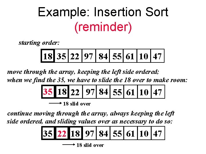
Example: Insertion Sort (reminder) starting order: 18 35 22 97 84 55 61 10 47 move through the array, keeping the left side ordered; when we find the 35, we have to slide the 18 over to make room: 35 18 22 97 84 55 61 10 47 18 slid over continue moving through the array, always keeping the left side ordered, and sliding values over as necessary to do so: 35 22 18 97 84 55 61 10 47 18 slid over

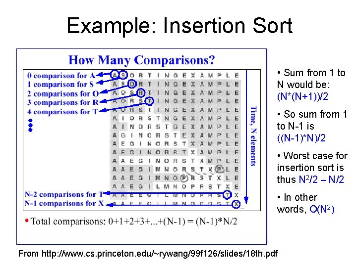
Example: Insertion Sort • Sum from 1 to N would be: (N*(N+1))/2 • So sum from 1 to N-1 is ((N-1)*N)/2 • Worst case for insertion sort is thus N 2/2 – N/2 • In other words, O(N 2) From http: //www. cs. princeton. edu/~rywang/99 f 126/slides/18 th. pdf

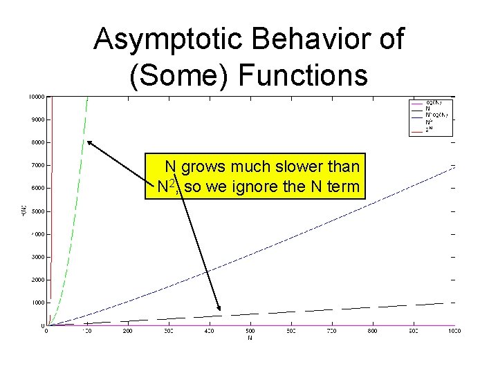
Asymptotic Behavior of (Some) Functions N grows much slower than N 2, so we ignore the N term

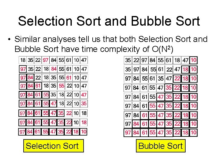
Selection Sort and Bubble Sort • Similar analyses tell us that both Selection Sort and Bubble Sort have time complexity of O(N 2) Selection Sort Bubble Sort

Some Complexity Examples For each of the following examples: 1. What task does the function perform? 2. What is the time complexity of the function? 3. Write a function which performs the same task but which is an order-ofmagnitude (not a constant factor) improvement in time complexity

Example 1 public int some. Method 1 (int[] a) { int temp = 0; for (int i=0; i < a. length; i++) for (int j=i+1; j < a. length; j++) if (Math. abs(a[j]-a[i]) > temp) temp = Math. abs(a[j]-a[i]); return temp; }

Example 1 public int some. Method 1 (int[] a) { int temp = 0; for (int i=0; i < a. length; i++) for (int j=i+1; j < a. length; j++) if (Math. abs(a[j]-a[i]) > temp) temp = Math. abs(a[j]-a[i]); return temp; } 1. Finds maximum difference between two values in the array

Example 1 public int some. Method 1 (int[] a) { int temp = 0; for (int i=0; i < a. length; i++) for (int j=i+1; j < a. length; j++) if (Math. abs(a[j]-a[i]) > temp) temp = Math. abs(a[j]-a[i]); return temp; } 1. Finds maximum difference between two values in the array 2. O(n 2)

Example 1 public int some. Method 1 (int[] a) { int temp = 0; for (int i=0; i < a. length; i++) for (int j=i+1; j < a. length; j++) if (Math. abs(a[j]-a[i]) > temp) temp = Math. abs(a[j]-a[i]); return temp; } 1. Finds maximum difference between two values in the array 2. O(n 2) 3. Find the max and min values in the array, then subtract one from the other – the problem will be solved in O(n)

Example 2: a[ ] is sorted in increasing order, b[ ] is not sorted public boolean some. Method 2(int[] a, int[] b) { for (int j=0; j < b. length; j++) for (int i=0; i < a. length-1; i++) if (b[j] == a[i] + a[i+1]) return true; return false; }

Example 2: a[ ] is sorted in increasing order, b[ ] is not sorted public boolean some. Method 2(int[] a, int[] b) { for (int j=0; j < b. length; j++) for (int i=0; i < a. length-1; i++) if (b[j] == a[i] + a[i+1]) return true; return false; } 1. Checks whether a value in b[ ] equals the sum of two consecutive values in a[ ]

Example 2: a[ ] is sorted in increasing order, b[ ] is not sorted public boolean some. Method 2(int[] a, int[] b) { for (int j=0; j < b. length; j++) for (int i=0; i < a. length-1; i++) if (b[j] == a[i] + a[i+1]) return true; return false; } 1. Checks whether a value in b[ ] equals the sum of two consecutive values in a[ ] 2. O(n 2)

Example 2: a[ ] is sorted in increasing order, b[ ] is not sorted public boolean some. Method 2(int[] a, int[] b) { for (int j=0; j < b. length; j++) for (int i=0; i < a. length-1; i++) if (b[j] == a[i] + a[i+1]) return true; return false; } 1. Checks whether a value in b[ ] equals the sum of two consecutive values in a[ ] 2. O(n 2) 3. For each value in b[ ], carry out a variation of a binary search in a[ ] – the problem will be solved in O(n log n)

Example 3: each element of a[ ] is a unique int between 1 and n; a. length is n-1 public int some. Method 3 (int[] a) { boolean flag; for (int j=1; j<=a. length+1; j++) { flag = false; for (int i=0; i<a. length; i++) { if (a[i]==j) { flag = true; break; } } if (!flag) return j; } return -1; }

Example 3: each element of a[ ] is a unique int between 1 and n; a. length is n-1 public int some. Method 3 (int[] a) { boolean flag; for (int j=1; j<=a. length+1; j++) { flag = false; for (int i=0; i<a. length; i++) { if (a[i]==j) { flag = true; break; } } if (!flag) return j; } return -1; } 1. Returns the missing value (the integer between 1 and n missing in a[ ])

Example 3: each element of a[ ] is a unique int between 1 and n; a. length is n-1 public int some. Method 3 (int[] a) { boolean flag; for (int j=1; j<=a. length+1; j++) { flag = false; for (int i=0; i<a. length; i++) { if (a[i]==j) { flag = true; break; } } if (!flag) return j; } return -1; } 1. Returns the missing value (the integer between 1 and n missing in a[ ]) 2. O(n 2)

A better solution to Example 3 public int better. Method 3 (int[] a) { int result = 0, sum, n; n = a. length+1; sum = (n*(n+1))/2; for (int i=0; i < a. length; i++) result += a[i]; return (sum-result); }

A better solution to Example 3 public int better. Method 3 (int[] a) { int result = 0, sum, n; n = a. length+1; sum = (n*(n+1))/2; for (int i=0; i < a. length; i++) result += a[i]; return (sum-result); } Time complexity O(n)

Theoretical Computer Science • Studies the complexity of problems: – increasing theoretical lower bound on the complexity of a problem – determining the worst-case and average-case complexity of a problem (along with bestcase) – showing that a problem falls into a given complexity class (e. g. , requires at least, or no more than, polynomial time)

Easy and Hard problems • “Easy” problems, by convention, are those that can be solved in polynomial time or less • “Hard” problems have only nonpolynomial solutions: exponential or worse • Showing that a problem is easy (come up with an “easy” algorithm); proving a problem is hard

Theory and algorithms • Theoretical computer scientists also – devise algorithms that take advantage of different kinds of computer hardware, like parallel processors – devise probabilistic algorithms that have very good average-case performance (though worst-case performance might be very bad) – narrow the gap between the inherent complexity of a problem and the best currently known algorithm for solving it