Algorithms Design and Complexity Analysis Algorithm Sequence of

Algorithms Design and Complexity Analysis

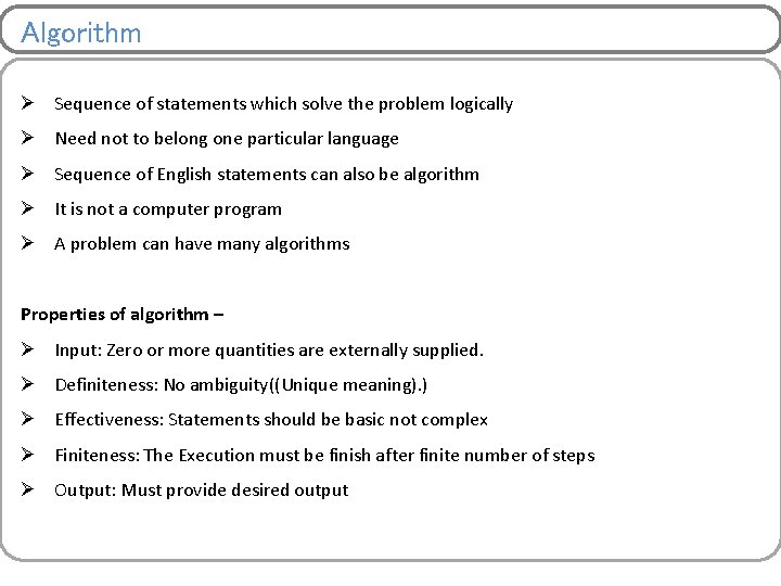
Algorithm Ø Sequence of statements which solve the problem logically Ø Need not to belong one particular language Ø Sequence of English statements can also be algorithm Ø It is not a computer program Ø A problem can have many algorithms Properties of algorithm – Ø Input: Zero or more quantities are externally supplied. Ø Definiteness: No ambiguity((Unique meaning). ) Ø Effectiveness: Statements should be basic not complex Ø Finiteness: The Execution must be finish after finite number of steps Ø Output: Must provide desired output

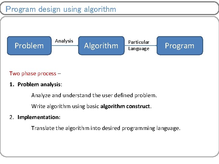
Program design using algorithm Problem Analysis Algorithm Particular Language Program Two phase process – 1. Problem analysis: Analyze and understand the user defined problem. Write algorithm using basic algorithm construct. 2. Implementation: Translate the algorithm into desired programming language.

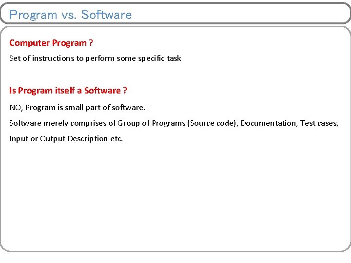
Program vs. Software Computer Program ? Set of instructions to perform some specific task Is Program itself a Software ? NO, Program is small part of software. Software merely comprises of Group of Programs (Source code), Documentation, Test cases, Input or Output Description etc.

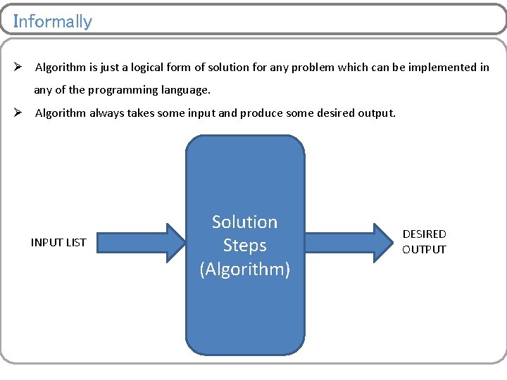
Informally Ø Algorithm is just a logical form of solution for any problem which can be implemented in any of the programming language. Ø Algorithm always takes some input and produce some desired output. INPUT LIST Solution Steps (Algorithm) DESIRED OUTPUT

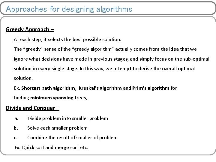
Approaches for designing algorithms Greedy Approach – At each step, it selects the best possible solution. The “greedy” sense of the “greedy algorithm” actually comes from the idea that we ignore what decisions have made in previous stages, and simply focus on the sub-optimal solution in every single stage. In this way, we attempt to derive the overall optimal solution. Ex. Shortest path algorithm, Kruskal's algorithm and Prim's algorithm for finding minimum spanning trees, Divide and Conquer – a. Divide problem into smaller problem b. Solve each smaller problem c. Combine the result of smaller of problem Ex. Quick sort and merge sort etc.

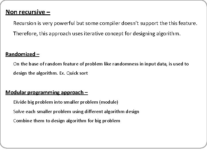
Non recursive – Recursion is very powerful but some compiler doesn’t support the this feature. Therefore, this approach uses iterative concept for designing algorithm. Randomized – On the base of random feature of problem like randomness in input data, is used to design the algorithm. Ex. Quick sort Modular programming approach – Divide big problem into smaller problem (module) Solve each smaller problem using different algorithm design Combine them to design algorithm for big problem

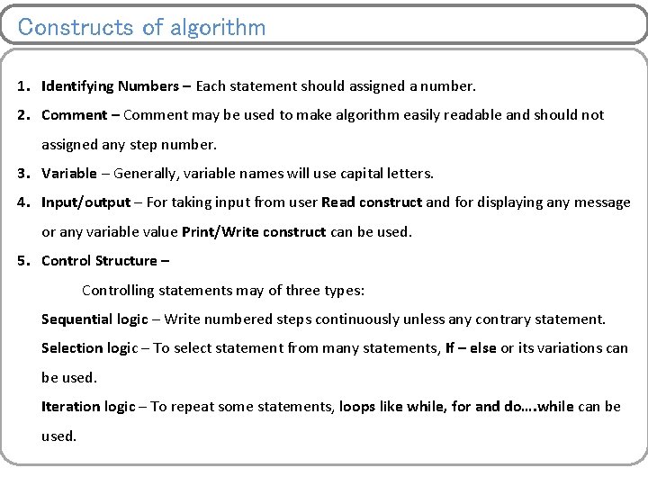
Constructs of algorithm 1. Identifying Numbers – Each statement should assigned a number. 2. Comment – Comment may be used to make algorithm easily readable and should not assigned any step number. 3. Variable – Generally, variable names will use capital letters. 4. Input/output – For taking input from user Read construct and for displaying any message or any variable value Print/Write construct can be used. 5. Control Structure – Controlling statements may of three types: Sequential logic – Write numbered steps continuously unless any contrary statement. Selection logic – To select statement from many statements, If – else or its variations can be used. Iteration logic – To repeat some statements, loops like while, for and do…. while can be used.

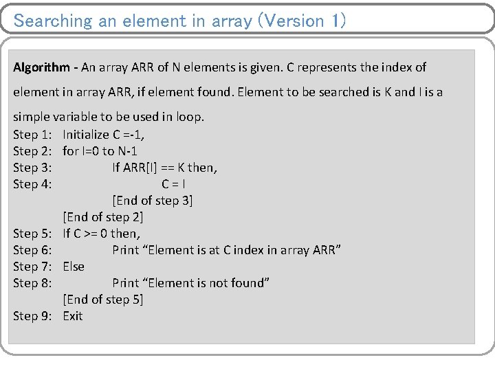
Searching an element in array (Version 1) Algorithm - An array ARR of N elements is given. C represents the index of element in array ARR, if element found. Element to be searched is K and I is a simple variable to be used in loop. Step 1: Initialize C =-1, Step 2: for I=0 to N-1 Step 3: If ARR[I] == K then, Step 4: C = I [End of step 3] [End of step 2] Step 5: If C >= 0 then, Step 6: Print “Element is at C index in array ARR” Step 7: Else Step 8: Print “Element is not found” [End of step 5] Step 9: Exit

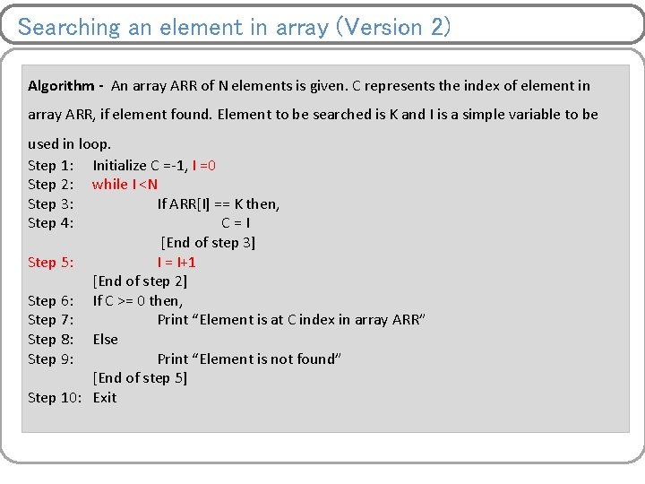
Searching an element in array (Version 2) Algorithm - An array ARR of N elements is given. C represents the index of element in array ARR, if element found. Element to be searched is K and I is a simple variable to be used in loop. Step 1: Initialize C =-1, I =0 Step 2: while I <N Step 3: If ARR[I] == K then, Step 4: C = I [End of step 3] Step 5: I = I+1 [End of step 2] Step 6: If C >= 0 then, Step 7: Print “Element is at C index in array ARR” Step 8: Else Step 9: Print “Element is not found” [End of step 5] Step 10: Exit

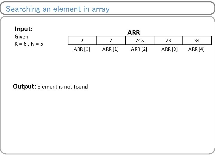
Searching an element in array Input: Given K = 6 , N = 5 ARR 7 2 243 23 34 ARR [0] ARR [1] ARR [2] ARR [3] ARR [4] Output: Element is not found

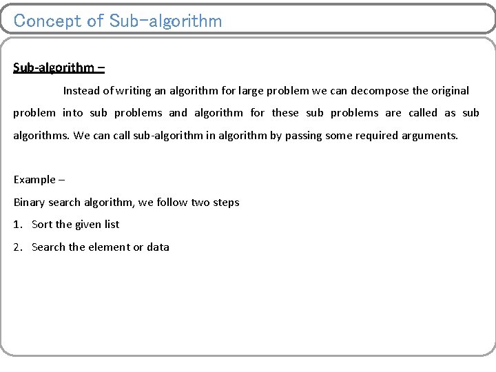
Concept of Sub-algorithm – Instead of writing an algorithm for large problem we can decompose the original problem into sub problems and algorithm for these sub problems are called as sub algorithms. We can call sub-algorithm in algorithm by passing some required arguments. Example – Binary search algorithm, we follow two steps 1. Sort the given list 2. Search the element or data

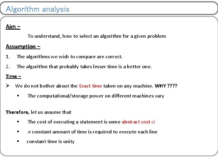
Algorithm analysis Aim – To understand, how to select an algorithm for a given problem Assumption – 1. The algorithms we wish to compare correct. 2. The algorithm that probably takes lesser time is a better one. Time – Ø We do not bother about the Exact time taken on any machine. WHY ? ? § The computational/storage power on different machines vary Therefore, let us assume that § The cost of executing a statement is some abstract cost ci § a constant amount of time is required to execute each line § constant time is unity

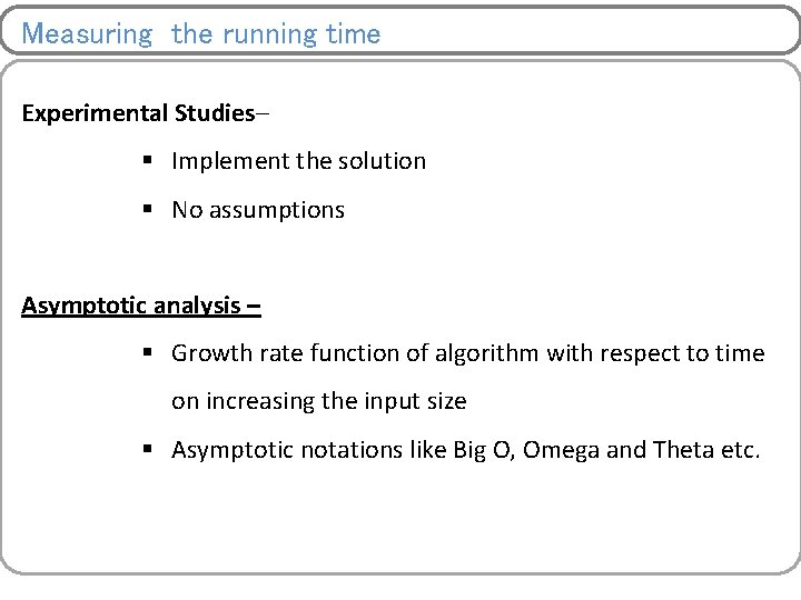
Measuring the running time Experimental Studies– § Implement the solution § No assumptions Asymptotic analysis – § Growth rate function of algorithm with respect to time on increasing the input size § Asymptotic notations like Big O, Omega and Theta etc.

Experimental Studies • Write a program implementing the algorithm • Run the program with inputs of varying size and composition. • Use a method like System. current. Time. Millis() to get an accurate measure of the actual running time 15

Limitations of Experiments • It is necessary to implement the algorithm, which may be difficult • Results may not be indicative of the running time on other inputs not included in the experiment. • In order to compare two algorithms, the same hardware and software environments must be used. 16

Beyond Experimental Studies– First we are going to develop a high level description of an algorithm. The way of describing an algorithm and we are going to use this description to figure out the running time such that we can get rid off from the limitation of the experimental studies approach: 1. No need to implement algorithm to any system. 2. A methodology would help us to take into account of all possible input instances and 3. also it will allow us to evaluate the efficiency of the algorithm in a way that it is independent of the platform we are using.

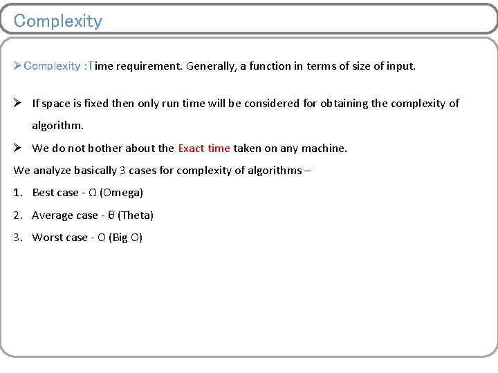
Complexity ØComplexity : Time requirement. Generally, a function in terms of size of input. Ø If space is fixed then only run time will be considered for obtaining the complexity of algorithm. Ø We do not bother about the Exact time taken on any machine. We analyze basically 3 cases for complexity of algorithms – 1. Best case - Ω (Omega) 2. Average case - θ (Theta) 3. Worst case - O (Big O)

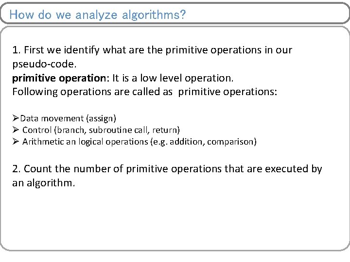
How do we analyze algorithms? 1. First we identify what are the primitive operations in our pseudo-code. primitive operation: It is a low level operation. Following operations are called as primitive operations: ØData movement (assign) Ø Control (branch, subroutine call, return) Ø Arithmetic an logical operations (e. g. addition, comparison) 2. Count the number of primitive operations that are executed by an algorithm.

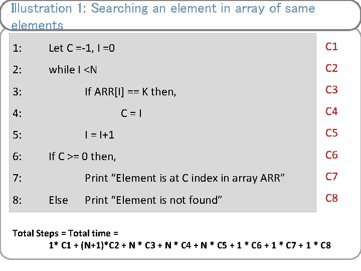
Illustration 1: Searching an element in array of same elements 1: Let C =-1, I =0 C 1 2: while I <N C 2 3: If ARR[I] == K then, C 3 4: C = I C 4 5: I = I+1 C 5 6: If C >= 0 then, C 6 7: 8: Else Print “Element is at C index in array ARR” C 7 Print “Element is not found” C 8 Total Steps = Total time = 1* C 1 + (N+1)*C 2 + N * C 3 + N * C 4 + N * C 5 + 1 * C 6 + 1 * C 7 + 1 * C 8

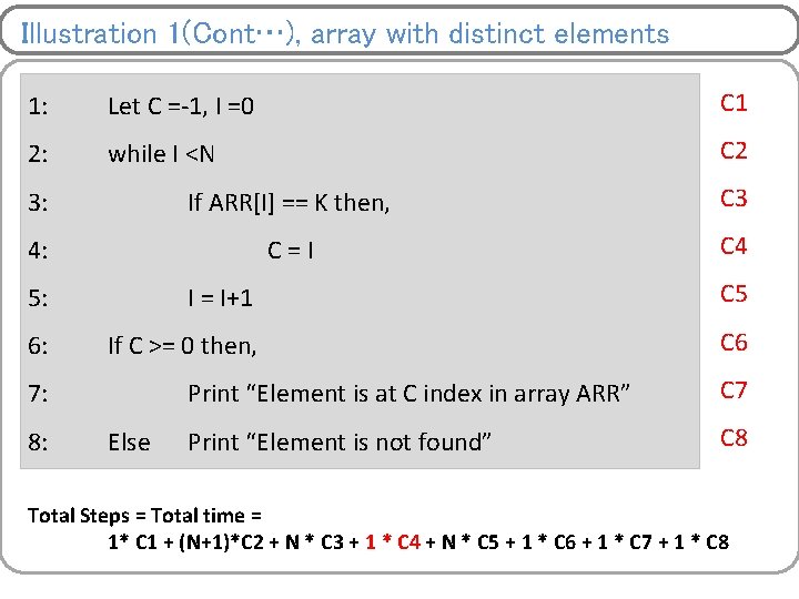
Illustration 1(Cont…), array with distinct elements 1: Let C =-1, I =0 C 1 2: while I <N C 2 3: If ARR[I] == K then, C 3 4: C = I C 4 5: I = I+1 C 5 6: If C >= 0 then, C 6 7: 8: Else Print “Element is at C index in array ARR” C 7 Print “Element is not found” C 8 Total Steps = Total time = 1* C 1 + (N+1)*C 2 + N * C 3 + 1 * C 4 + N * C 5 + 1 * C 6 + 1 * C 7 + 1 * C 8

Illustration 2: Largest Element in array 1: let max = x[0] C 1 2: for i = 1 to n-1 C 2 3: C 3 4: 5: Print max if x[i] > max then, max = x[i] Descending Order – Total Steps = Total time = 1* C 1 + n*C 2 + (n-1 )* C 3 + 1* C 5 Ascending Order – Total Steps = Total time = 1* C 1 + n*C 2 + (n-1 )* C 3 + (n-1) * C 4 + 1* C 5 C 4 C 5

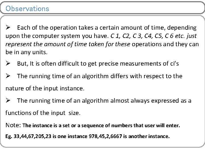
Observations Ø Each of the operation takes a certain amount of time, depending upon the computer system you have. C 1, C 2, C 3, C 4, C 5, C 6 etc. just represent the amount of time taken for these operations and they can be in any units. Ø But, It is often difficult to get precise measurements of ci’s Ø The running time of an algorithm differs with respect to the nature of the input instance. Ø The running time of an algorithm almost always expressed as a functions of the input size. Note: The instance is a set or a sequence of numbers that user will enter. Eg. 33, 44, 67, 205, 23 is one instance 978, 45, 2, 6667 is another instance.

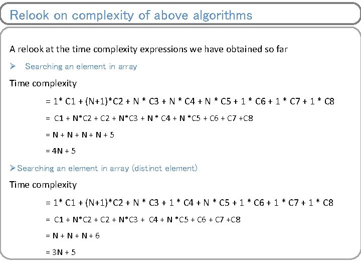
Relook on complexity of above algorithms A relook at the time complexity expressions we have obtained so far Ø Searching an element in array Time complexity = 1* C 1 + (N+1)*C 2 + N * C 3 + N * C 4 + N * C 5 + 1 * C 6 + 1 * C 7 + 1 * C 8 = C 1 + N*C 2 + N*C 3 + N * C 4 + N *C 5 + C 6 + C 7 +C 8 = N + N + 5 = 4 N + 5 ØSearching an element in array (distinct element) Time complexity = 1* C 1 + (N+1)*C 2 + N * C 3 + 1 * C 4 + N * C 5 + 1 * C 6 + 1 * C 7 + 1 * C 8 = C 1 + N*C 2 + N*C 3 + C 4 + N *C 5 + C 6 + C 7 +C 8 = N + N + 6 = 3 N + 5

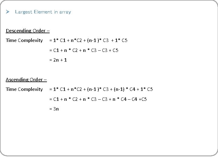
Ø Largest Element in array Descending Order – Time Complexity = 1* C 1 + n*C 2 + (n-1 )* C 3 + 1* C 5 = C 1 + n * C 2 + n * C 3 – C 3 + C 5 = 2 n + 1 Ascending Order – Time Complexity = 1* C 1 + n*C 2 + (n-1 )* C 3 + (n-1) * C 4 + 1* C 5 = C 1 + n * C 2 + n * C 3 – C 3 + n * C 4 – C 4 +C 5 = 3 n

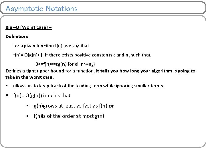
Asymptotic Notations Ø Asymptotic notation is a way of expressing the cost of an algorithm. Ø Goal of Asymptotic notation is to simplify Analysis by getting rid of unneeded information

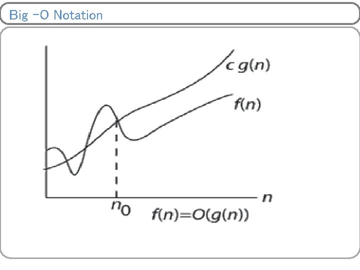
Asymptotic Notations Big –O (Worst Case) – Definition: for a given function f(n), we say that f(n)= O(g(n)) | if there exists positive constants c and no such that, 0<=f(n)<=cg(n) for all n>=no} Defines a tight upper bound for a function, it tells you how long your algorithm is going to take in the worst case. § allows us to keep track of the leading term while ignoring smaller terms § f(n)= O(g(n)) implies that § g(n)grows at least as f(n) or § f(n)is of the order at most g(n)

Big –O Notation

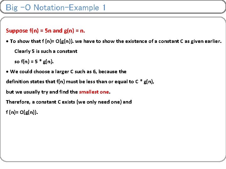
Big –O Notation-Example 1 Suppose f(n) = 5 n and g(n) = n. • To show that f (n)= O(g(n)). we have to show the existence of a constant C as given earlier. Clearly 5 is such a constant so f(n) = 5 * g(n). • We could choose a larger C such as 6, because the definition states that f(n) must be less than or equal to C * g(n), but we usually try and find the smallest one. Therefore, a constant C exists (we only need one) and f (n)= O(g(n)).

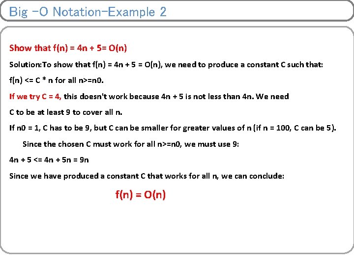
Big –O Notation-Example 2 Show that f(n) = 4 n + 5= O(n) Solution: To show that f(n) = 4 n + 5 = O(n), we need to produce a constant C such that: f(n) <= C * n for all n>=n 0. If we try C = 4, this doesn't work because 4 n + 5 is not less than 4 n. We need C to be at least 9 to cover all n. If n 0 = 1, C has to be 9, but C can be smaller for greater values of n (if n = 100, C can be 5). Since the chosen C must work for all n>=n 0, we must use 9: 4 n + 5 <= 4 n + 5 n = 9 n Since we have produced a constant C that works for all n, we can conclude: f(n) = O(n)

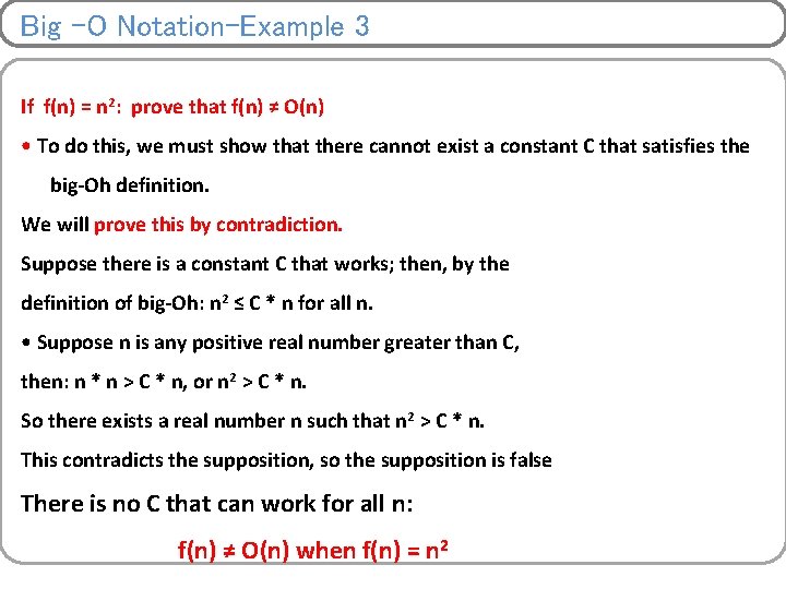
Big –O Notation-Example 3 If f(n) = n 2: prove that f(n) ≠ O(n) • To do this, we must show that there cannot exist a constant C that satisfies the big-Oh definition. We will prove this by contradiction. Suppose there is a constant C that works; then, by the definition of big-Oh: n 2 ≤ C * n for all n. • Suppose n is any positive real number greater than C, then: n * n > C * n, or n 2 > C * n. So there exists a real number n such that n 2 > C * n. This contradicts the supposition, so the supposition is false There is no C that can work for all n: f(n) ≠ O(n) when f(n) = n 2

Big –O Notation

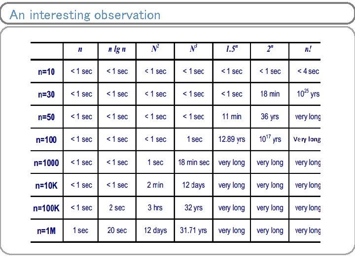
An interesting observation Very long

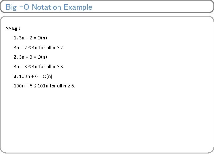
Big –O Notation Example >> Eg : 1. 3 n + 2 = O(n) 3 n + 2 ≤ 4 n for all n ≥ 2. 2. 3 n + 3 = O(n) 3 n + 3 ≤ 4 n for all n ≥ 3. 3. 100 n + 6 = O(n) 100 n + 6 ≤ 101 n for all n ≥ 6.

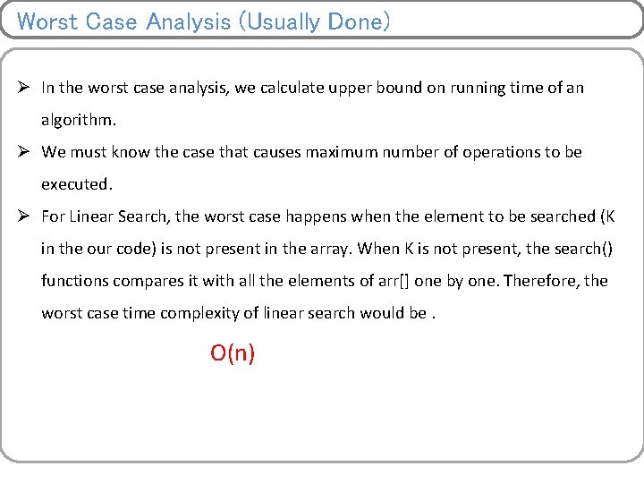
Worst Case Analysis (Usually Done) Ø In the worst case analysis, we calculate upper bound on running time of an algorithm. Ø We must know the case that causes maximum number of operations to be executed. Ø For Linear Search, the worst case happens when the element to be searched (K in the our code) is not present in the array. When K is not present, the search() functions compares it with all the elements of arr[] one by one. Therefore, the worst case time complexity of linear search would be. O(n)

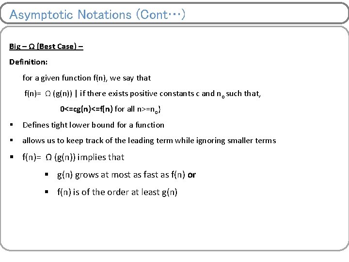
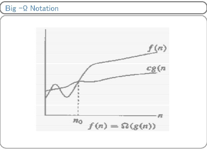
Asymptotic Notations (Cont…) Big – Ω (Best Case) – Definition: for a given function f(n), we say that f(n)= Ω (g(n)) | if there exists positive constants c and no such that, 0<=cg(n)<=f(n) for all n>=no} § Defines tight lower bound for a function § allows us to keep track of the leading term while ignoring smaller terms § f(n)= Ω (g(n)) implies that § g(n) grows at most as fast as f(n) or § f(n) is of the order at least g(n)

Big –Ω Notation

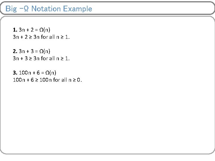
Big –Ω Notation Example 1. 3 n + 2 = Ω(n) 3 n + 2 ≥ 3 n for all n ≥ 1. 2. 3 n + 3 = Ω(n) 3 n + 3 ≥ 3 n for all n ≥ 1. 3. 100 n + 6 = Ω(n) 100 n + 6 ≥ 100 n for all n ≥ 0.

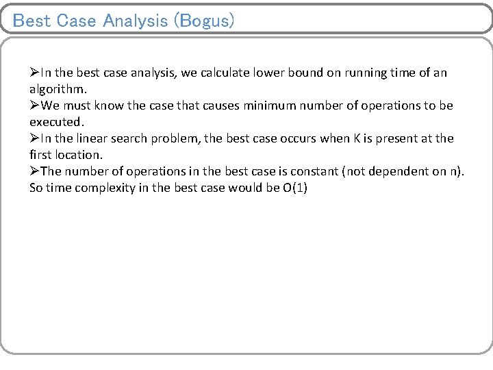
Best Case Analysis (Bogus) ØIn the best case analysis, we calculate lower bound on running time of an algorithm. ØWe must know the case that causes minimum number of operations to be executed. ØIn the linear search problem, the best case occurs when K is present at the first location. ØThe number of operations in the best case is constant (not dependent on n). So time complexity in the best case would be O(1)

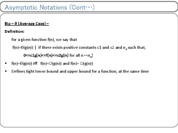
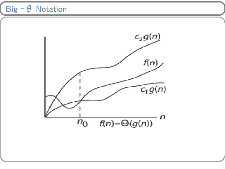
Asymptotic Notations (Cont…) Big – θ (Average Case) – Definition: for a given function f(n), we say that f(n)=θ(g(n)) | if there exists positive constants c 1 and c 2 and no such that, 0<=c 1 g(n)<=f(n)<=c 2 g(n) for all n>=no} § f(n)=θ(g(n)) iff f(n)=O(g(n)) and f(n)= Ω(g(n)) § Defines tight lower bound and upper bound for a function, at the same time

Big –θ Notation

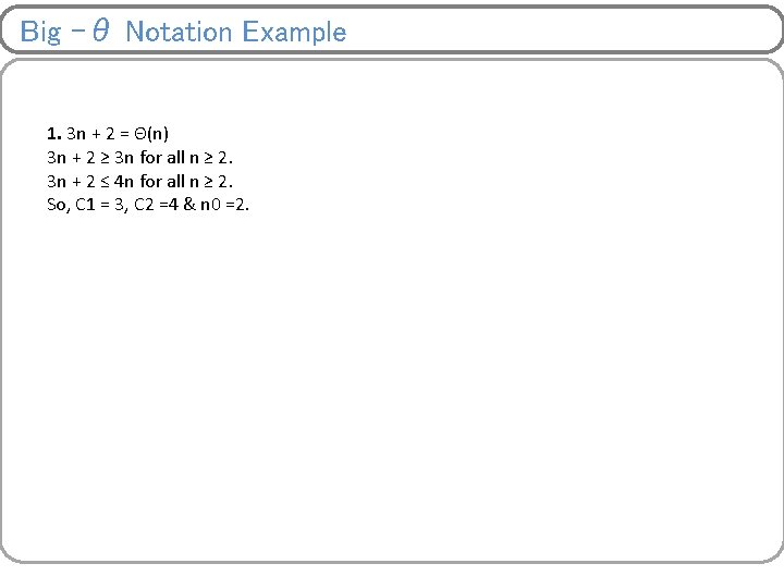
Big –θ Notation Example 1. 3 n + 2 = Θ(n) 3 n + 2 ≥ 3 n for all n ≥ 2. 3 n + 2 ≤ 4 n for all n ≥ 2. So, C 1 = 3, C 2 =4 & n 0 =2.

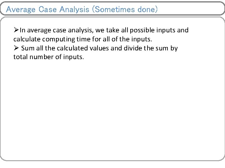
Average Case Analysis (Sometimes done) ØIn average case analysis, we take all possible inputs and calculate computing time for all of the inputs. Ø Sum all the calculated values and divide the sum by total number of inputs.

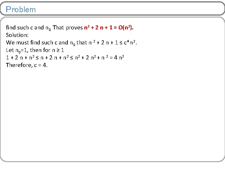
Problem find such c and n 0 That proves n 2 + 2 n + 1 = O(n 2). Solution: We must find such c and n 0 that n 2 + 2 n + 1 ≤ c*n 2. Let n 0=1, then for n ≥ 1 1 + 2 n + n 2 ≤ n 2 + 2 n 2 + n 2 = 4 n 2 Therefore, c = 4.

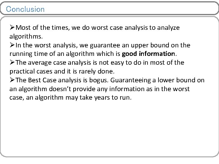
Conclusion ØMost of the times, we do worst case analysis to analyze algorithms. ØIn the worst analysis, we guarantee an upper bound on the running time of an algorithm which is good information. ØThe average case analysis is not easy to do in most of the practical cases and it is rarely done. ØThe Best Case analysis is bogus. Guaranteeing a lower bound on an algorithm doesn’t provide any information as in the worst case, an algorithm may take years to run.

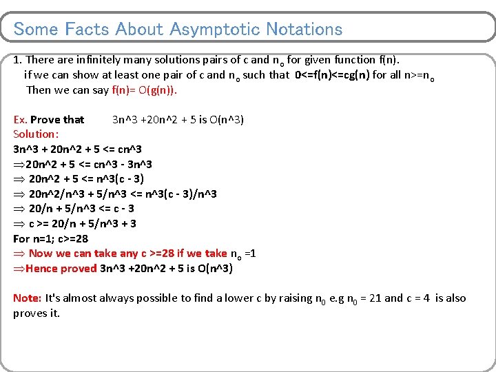
Some Facts About Asymptotic Notations 1. There are infinitely many solutions pairs of c and no for given function f(n). if we can show at least one pair of c and no such that 0<=f(n)<=cg(n) for all n>=no Then we can say f(n)= O(g(n)). Ex. Prove that 3 n^3 +20 n^2 + 5 is O(n^3) Solution: 3 n^3 + 20 n^2 + 5 <= cn^3 Þ 20 n^2 + 5 <= cn^3 - 3 n^3 Þ 20 n^2 + 5 <= n^3(c - 3) Þ 20 n^2/n^3 + 5/n^3 <= n^3(c - 3)/n^3 Þ 20/n + 5/n^3 <= c - 3 Þ c >= 20/n + 5/n^3 + 3 For n=1; c>=28 Þ Now we can take any c >=28 if we take no =1 ÞHence proved 3 n^3 +20 n^2 + 5 is O(n^3) Note: It's almost always possible to find a lower c by raising n 0 e. g n 0 = 21 and c = 4 is also proves it.

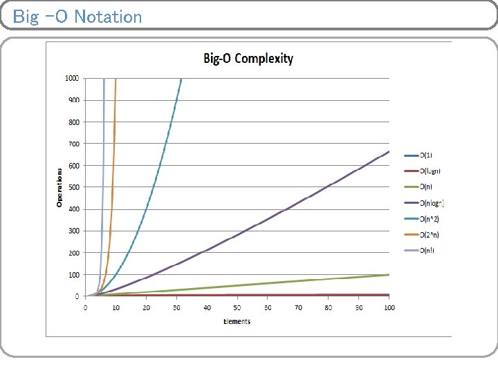
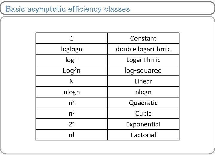
Basic asymptotic efficiency classes 1 loglogn Constant double logarithmic Log 2 n N nlogn n 2 n 3 2 n n! log-squared Linear nlogn Quadratic Cubic Exponential Factorial

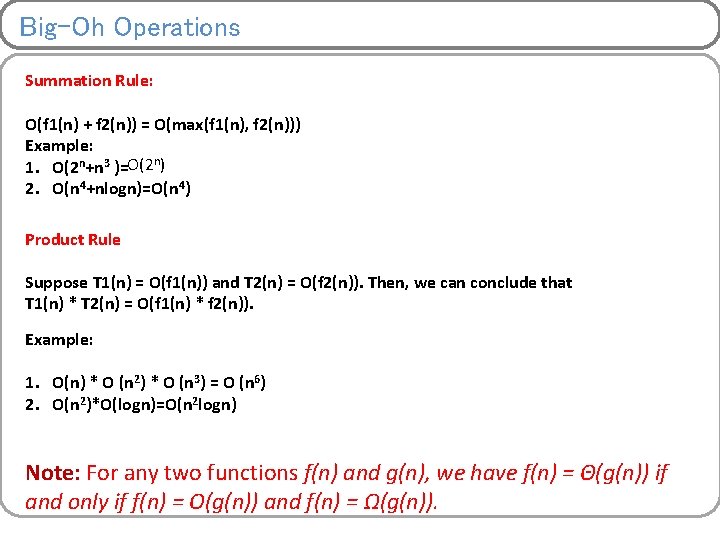
Big-Oh Operations Summation Rule: O(f 1(n) + f 2(n)) = O(max(f 1(n), f 2(n))) Example: 1. O(2 n+n 3 )=O(2 n) 2. O(n 4+nlogn)=O(n 4) Product Rule Suppose T 1(n) = O(f 1(n)) and T 2(n) = O(f 2(n)). Then, we can conclude that T 1(n) * T 2(n) = O(f 1(n) * f 2(n)). Example: 1. O(n) * O (n 2) * O (n 3) = O (n 6) 2. O(n 2)*O(logn)=O(n 2 logn) Note: For any two functions f(n) and g(n), we have f(n) = Θ(g(n)) if and only if f(n) = O(g(n)) and f(n) = Ω(g(n)).

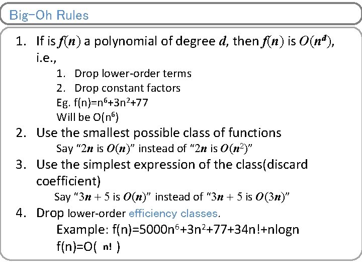
Big-Oh Rules 1. If is f(n) a polynomial of degree d, then f(n) is O(nd), i. e. , 1. Drop lower-order terms 2. Drop constant factors Eg. f(n)=n 6+3 n 2+77 Will be O(n 6) 2. Use the smallest possible class of functions Say “ 2 n is O(n)” instead of “ 2 n is O(n 2)” 3. Use the simplest expression of the class(discard coefficient) Say “ 3 n + 5 is O(n)” instead of “ 3 n + 5 is O(3 n)” 4. Drop lower-order efficiency classes. Example: f(n)=5000 n 6+3 n 2+77+34 n!+nlogn n! f(n)=O( )

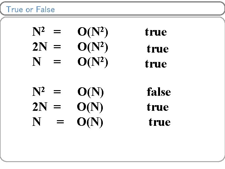
True or False N 2 = 2 N = O(N 2) true N 2 = 2 N = O(N) false true

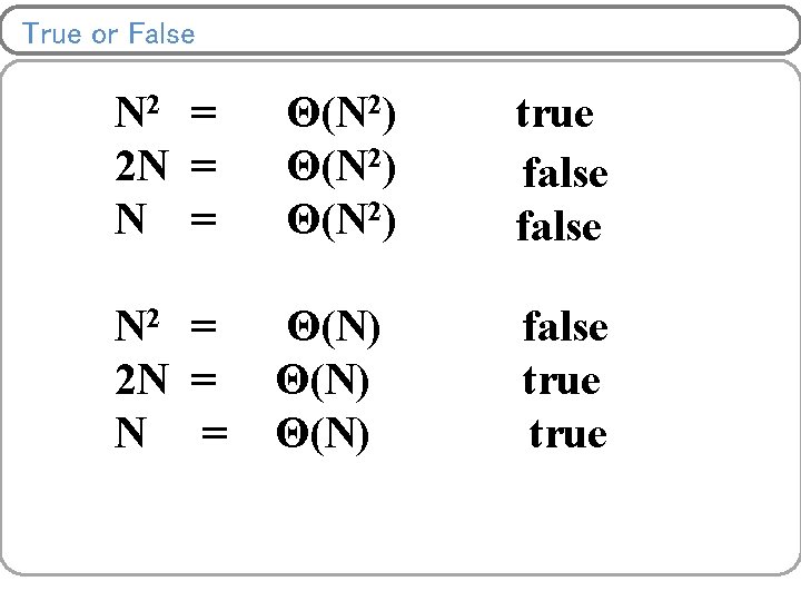
True or False N 2 = 2 N = Θ(N 2) true false N 2 = 2 N = Θ(N) false true

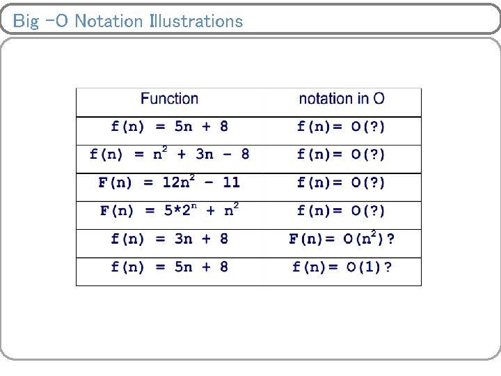
Big –O Notation Illustrations

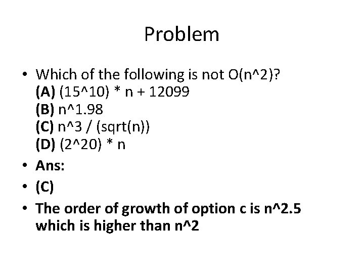
Problem • Which of the following is not O(n^2)? (A) (15^10) * n + 12099 (B) n^1. 98 (C) n^3 / (sqrt(n)) (D) (2^20) * n • Ans: • (C) • The order of growth of option c is n^2. 5 which is higher than n^2

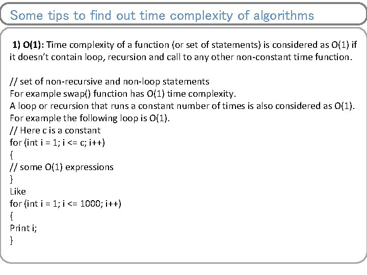
Some tips to find out time complexity of algorithms 1) O(1): Time complexity of a function (or set of statements) is considered as O(1) if it doesn’t contain loop, recursion and call to any other non-constant time function. // set of non-recursive and non-loop statements For example swap() function has O(1) time complexity. A loop or recursion that runs a constant number of times is also considered as O(1). For example the following loop is O(1). // Here c is a constant for (int i = 1; i <= c; i++) { // some O(1) expressions } Like for (int i = 1; i <= 1000; i++) { Print i; }

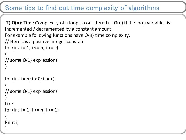
Some tips to find out time complexity of algorithms 2) O(n): Time Complexity of a loop is considered as O(n) if the loop variables is incremented / decremented by a constant amount. For example following functions have O(n) time complexity. // Here c is a positive integer constant for (int i = 1; i <= n; i += c) { // some O(1) expressions } for (int i = n; i > 0; i -= c) { // some O(1) expressions } Like for (int i = 1; i <= n; i += 1) { Print i; }

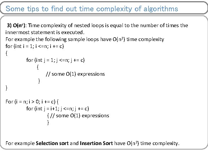
Some tips to find out time complexity of algorithms 3) O(nc): Time complexity of nested loops is equal to the number of times the innermost statement is executed. For example the following sample loops have O(n 2) time complexity for (int i = 1; i <=n; i += c) { for (int j = 1; j <=n; j += c) { // some O(1) expressions } } For (i = n; i > 0; i += c) { for (int j = i+1; j <=n; j += c) { // some O(1) expressions } For example Selection sort and Insertion Sort have O(n 2) time complexity.

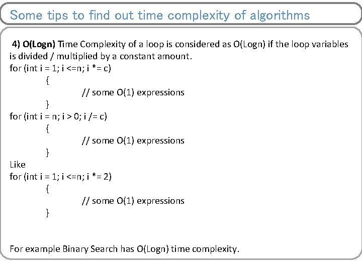
Some tips to find out time complexity of algorithms 4) O(Logn) Time Complexity of a loop is considered as O(Logn) if the loop variables is divided / multiplied by a constant amount. for (int i = 1; i <=n; i *= c) { // some O(1) expressions } for (int i = n; i > 0; i /= c) { // some O(1) expressions } Like for (int i = 1; i <=n; i *= 2) { // some O(1) expressions } For example Binary Search has O(Logn) time complexity.

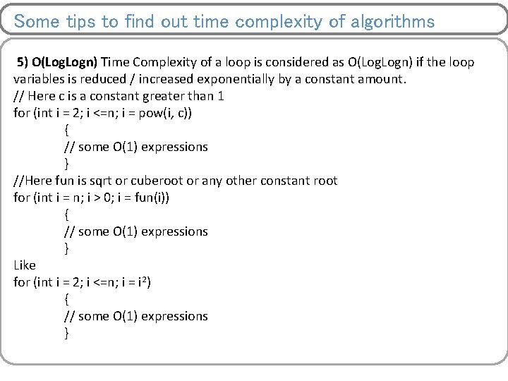
Some tips to find out time complexity of algorithms 5) O(Log. Logn) Time Complexity of a loop is considered as O(Log. Logn) if the loop variables is reduced / increased exponentially by a constant amount. // Here c is a constant greater than 1 for (int i = 2; i <=n; i = pow(i, c)) { // some O(1) expressions } //Here fun is sqrt or cuberoot or any other constant root for (int i = n; i > 0; i = fun(i)) { // some O(1) expressions } Like for (int i = 2; i <=n; i = i 2) { // some O(1) expressions }

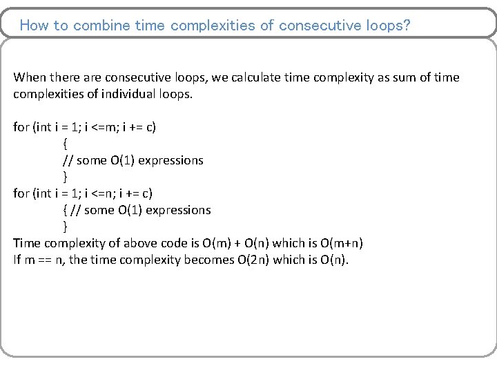
How to combine time complexities of consecutive loops? When there are consecutive loops, we calculate time complexity as sum of time complexities of individual loops. for (int i = 1; i <=m; i += c) { // some O(1) expressions } for (int i = 1; i <=n; i += c) { // some O(1) expressions } Time complexity of above code is O(m) + O(n) which is O(m+n) If m == n, the time complexity becomes O(2 n) which is O(n).

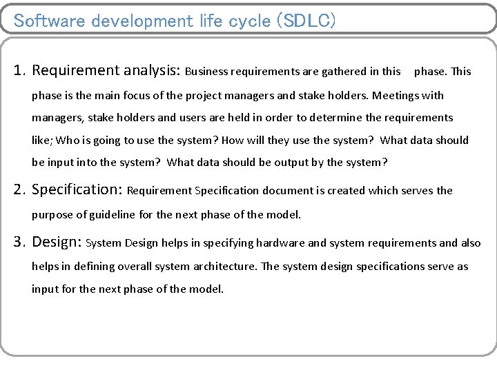
Software development life cycle (SDLC) 1. Requirement analysis: Business requirements are gathered in this phase. This phase is the main focus of the project managers and stake holders. Meetings with managers, stake holders and users are held in order to determine the requirements like; Who is going to use the system? How will they use the system? What data should be input into the system? What data should be output by the system? 2. Specification: Requirement Specification document is created which serves the purpose of guideline for the next phase of the model. 3. Design: System Design helps in specifying hardware and system requirements and also helps in defining overall system architecture. The system design specifications serve as input for the next phase of the model.

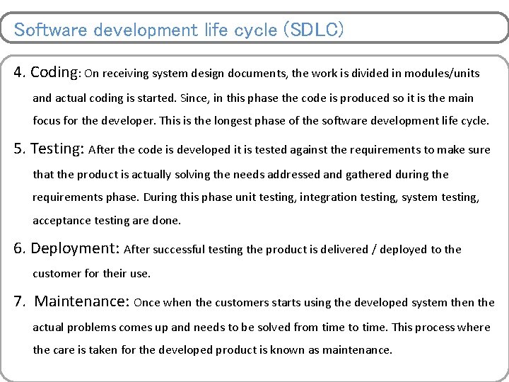
Software development life cycle (SDLC) 4. Coding: On receiving system design documents, the work is divided in modules/units and actual coding is started. Since, in this phase the code is produced so it is the main focus for the developer. This is the longest phase of the software development life cycle. 5. Testing: After the code is developed it is tested against the requirements to make sure that the product is actually solving the needs addressed and gathered during the requirements phase. During this phase unit testing, integration testing, system testing, acceptance testing are done. 6. Deployment: After successful testing the product is delivered / deployed to the customer for their use. 7. Maintenance: Once when the customers starts using the developed system then the actual problems comes up and needs to be solved from time to time. This process where the care is taken for the developed product is known as maintenance.