Artificial Intelligence Search Problem Search Problem Search is

Artificial Intelligence Search Problem

Search Problem Search is a problem-solving technique to explores successive stages in problemsolving process.

Search Space • We need to define a space to search in to find a problem solution • To successfully design and implement search algorithm, we must be able to analyze and predict its behavior.

State Space Search One tool to analyze the search space is to represent it as space graph, so by use graph theory we analyze the problem and solution of it.

Graph Theory A graph consists of a set of nodes and a set of arcs or links connecting pairs of nodes. River 2 Island 1 Island 2 River 1

Graph structure • Nodes = {a, b, c, d, e} • Arcs = {(a, b), (a, d), (b, c), …. } d b c e a

Tree • A tree is a graph in which two nodes have at most one path between them. • The tree has a root. a b e f c g h d i j

Space representation In the space representation of a problem, the nodes of a graph correspond to partial problem solution states and arcs correspond to steps in a problem-solving process

Example • Let the game of Tic-Tac-toe 1 2 8 7 3 4 6 5

1 2 3 8 4 7 6 5 1 2 3 1 4 3 7 4 6 8 7 6 7 8 6 7 6 4 5 8 2 5 6 2 5 8 2 1 1 3 3 1 4 3 7 4 6 1 7 6 5 8 2 7 8 2

A simple example: traveling on a graph C 2 2 start state A 9 B 3 3 D 4 E F goal state 4

Search tree state = A, cost = 0 state = B, cost = 3 state = C, cost = 5 state = D, cost = 3 state = F, cost = 12 goal state! state = A, cost = 7 search tree nodes and states are not the same thing!

Full search tree state = A, cost = 0 state = B, cost = 3 state = C, cost = 5 state = F, cost = 12 state = D, cost = 3 state = E, cost = 7 goal state! state = A, cost = 7 state = F, cost = 11 goal state! . . . state = B, cost = 10 . . . state = D, cost = 10

Problem types • Deterministic, fully observable single-state problem – Solution is a sequence of states • Non-observable sensorless problem – Problem-solving may have no idea where it is; solution is a sequence • Nondeterministic and/or partially observable Unknown state space

Algorithm types • There are two kinds of search algorithm – Complete • guaranteed to find solution or prove there is none – Incomplete • may not find a solution even when it exists • often more efficient (or there would be no point)

Comparing Searching Algorithms: Will it find a solution? the best one? Def. : A search algorithm is complete if whenever there is at least one solution, the algorithm is guaranteed to find it within a finite amount of time. Def. : A search algorithm is optimal if when it finds a solution, it is the best one

Comparing Searching Algorithms: Complexity Branching factor b of a node is the number of arcs going out of the node Def. : The time complexity of a search algorithm is the worst- case amount of time it will take to run, expressed in terms of • maximum path length m • maximum branching factor b. Def. : The space complexity of a search algorithm is the worst-case amount of memory that the algorithm will use (i. e. , the maximum number of nodes on the frontier), also expressed in terms of m and b.

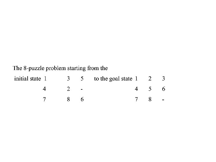
Example: the 8 -puzzle. Given: a board situation for the 8 puzzle: 1 3 8 2 5 7 4 6 Problem: find a sequence of moves that transform this board situation in a desired goal situation: 1 2 3 1 8 7 2 6 3 4 5

State Space representation In the space representation of a problem, the nodes of a graph correspond to partial problem solution states and arcs correspond to steps (action) in a problem-solving process

Key concepts in search • Set of states that we can be in – Including an initial state… – … and goal states (equivalently, a goal test) • For every state, a set of actions that we can take – Each action results in a new state – Given a state, produces all states that can be reached from it • Cost function that determines the cost of each action (or path = sequence of actions) • Solution: path from initial state to a goal state – Optimal solution: solution with minimal cost

0 ( New. York ) 250 ( New. York, Boston ) 1450 1700 ( New. York, Boston, Miami ) 1200 ( New. York, Miami ) 1500 2900 1500 ( New. York, Dallas ) 2900 ( New. York, Frisco ) 3300 6200 ( New. York, Frisco, Miami ) Keep track of accumulated costs in each state if you want to be sure to get the best path.

Example: Route Finding • Initial state – City journey starts in • Operators – Driving from city to city • Goal test Liverpool Leeds Nottingham Manchester Birmingham – Is current location the destination city? London

State space representation (salesman) • State: – the list of cities that are already visited • Ex. : ( New. York, Boston ) • Initial state: • Ex. : ( New. York ) • Rules: – add 1 city to the list that is not yet a member – add the first city if you already have 5 members • Goal criterion: – first and last city are equal

Example: The 8 -puzzle • • states? locations of tiles actions? move blank left, right, up, down goal? = goal state (given) path cost? 1 per move

Example: robotic assembly • states? : real-valued coordinates of robot joint angles parts of the object to be assembled • actions? : continuous motions of robot joints • goal test? : complete assembly • path cost? : time to execute

1 2 3 8 4 7 1 3 1 6 4 3 1 4 7 6 7 8 6 7 6 8 2 5 8 2 7 4 6 5 8 2 1 3 7 4 6 5 8 2 5 5 3 4 3 1 7 6 5 8 2

Example: Chess • Problem: develop a program that plays chess 1. A way to represent board situations l 8 7 6 5 4 3 2 1 Ex. : List: (( king_black, 8, C), ( knight_black, 7, B), ( pawn_black, 7, G), ( pawn_black, 5, F), ( pawn_white, 2, H), ( king_white, 1, E)) A B C D E F G H

Chess ~15 ~ (15)2 ~ (15)3 search tree Move 1 Move 2 Move 3 Need very efficient search techniques to find good paths in such combinatorial trees.

independence of states: Ex. : Blocks world problem. • Initially: C is on A and B is on the table. • Rules: to move any free block to another or to the table • Goal: A is on B and B is on C. C A AND-OR-tree? B Goal: A on B and B on C AND C A B Goal: A on B C A B Goal: B on C

Search in State Spaces • Effects of moving a block (illustration and list-structure iconic model notation)

Avoiding Repeated States • In increasing order of effectiveness in reducing size of state space and with increasing computational costs: 1. Do not return to the state you just came from. 2. Do not create paths with cycles in them. 3. Do not generate any state that was ever created before. • Net effect depends on frequency of “loops” in state space.

Forward versus backward reasoning: Initial states Goal states Forward reasoning (or Data-driven): from initial states to goal states.

Forward versus backward reasoning: Initial states Goal states Backward reasoning (or backward chaining / goal-driven ): from goal states

Data-Driven search • It is called forward chaining • The problem solver begins with the given facts and a set of legal moves or rules for changing state to arrive to the goal.

Goal-Driven Search • Take the goal that we want to solve and see what rules or legal moves could be used to generate this goal. • So we move backward.

Search Implementation • In both types of moving search, we must find the path from start state to a goal. • We use goal-driven search if – The goal is given in the problem – There exist a large number of rules – Problem data are not given

Search Implementation • The data-driven search is used if – All or most data are given – There a large number of potential goals – It is difficult to form a goal

Criteria: Sometimes equivalent: 1 3 2 5 8 7 4 6 1 8 7 2 6 3 4 5 In this case: even the same rules !! • Sometimes: no way to start from the goal states – because there are too many (Ex. : chess) – because you can’t (easily) formulate the rules in 2 directions.

General Search Considerations • Given initial state, operators and goal test – Can you give the agent additional information? • Uninformed search strategies – Have no additional information • Informed search strategies – Uses problem specific information – Heuristic measure (Guess how far from goal)

Classical Search Strategies Breadth-first search Depth-first search Bidirectional search Depth-bounded depth first search – like depth first but set limit on depth of search in tree • Iterative Deepening search – use depth-bounded search but iteratively increase limit • •

Breadth-first search: S D A B C E D D A E B F G C E B E A F C G F G It explores the space in a level-by-level fashion. • Move downward s, level by level, until goal is reached.

Breadth-first search • BFS is complete: if a solution exists, one will be found • Expand shallowest unexpanded node • Implementation: – fringe is a FIFO queue, i. e. , new successors go at end

Breadth-first search • Expand shallowest unexpanded node • Implementation: – fringe is a FIFO queue, i. e. , new successors go at end

Analysis of BFS Def. : A search algorithm is complete if whenever there is at least one solution, the algorithm is guaranteed to find it within a finite amount of time. Is BFS complete? Yes • If a solution exists at level l, the path to it will be explored before any other path of length l + 1 • impossible to fall into an infinite cycle • see this in AISpace by loading “Cyclic Graph Examples” or by adding a cycle to “Simple Tree” 46

Analysis of BFS Def. : A search algorithm is optimal if when it finds a solution, it is the best one Is BFS optimal? Yes • E. g. , two goal nodes: red boxes • Any goal at level l (e. g. red box N 7) will be reached before goals at lower levels 47

Analysis of BFS Def. : The time complexity of a search algorithm is the worst-case amount of time it will take to run, expressed in terms of - maximum path length m - maximum forward branching factor b. • What is BFS’s time complexity, in terms of m and b ? O(bm) • Like DFS, in the worst case BFS must examine every node in the tree • E. g. , single goal node -> red box 48

Analysis of BFS Def. : The space complexity of a search algorithm is the worst case amount of memory that the algorithm will use (i. e. , the maximal number of nodes on the frontier), expressed in terms of - maximum path length m - maximum forward branching factor b. • What is BFS’s space complexity, in terms of m and b ? O(bm) - BFS must keep paths to all the nodes al level m 49

Using Breadth-first Search • When is BFS appropriate? • space is not a problem • it's necessary to find the solution with the fewest arcs • When there are some shallow solutions • there may be infinite paths • When is BFS inappropriate? • space is limited • all solutions tend to be located deep in the tree • the branching factor is very large

Depth-First Order • When a state is examined, all of its children and their descendants are examined before any of its siblings. • Not complete (might cycle through nongoal states) • Depth- First order goes deeper whenever this is possible.

Depth-first search = Chronological backtracking S A B C E D F G • Select a child – convention: left-to-right • Repeatedly go to next child, as long as possible. • Return to left-over alternatives (higher-up) only when needed.

Depth-first search • Expand deepest unexpanded node • Implementation: – fringe = LIFO queue, i. e. , put successors at front

• Is DFS complete? Analysis of DFS . • Is DFS optimal? • What is the time complexity, if the maximum path length is m and the maximum branching factor is b ? • What is the space complexity? We will look at the answers in AISpace (but see next few slides for a summary of what we do)

Analysis of DFS Def. : A search algorithm is complete if whenever there is at least one solution, the algorithm is guaranteed to find it within a finite amount of time. No Is DFS complete? • If there are cycles in the graph, DFS may get “stuck” in one of them • see this in AISpace by loading “Cyclic Graph Examples” or by adding a cycle to “Simple Tree” • e. g. , click on “Create” tab, create a new edge from N 7 to N 1, go back to “Solve” and see what happens

Analysis of DFS Def. : A search algorithm is optimal if when it finds a solution, it is the best one (e. g. , the shortest) Is DFS optimal? No • It can “stumble” on longer solution paths before it gets to shorter ones. • E. g. , goal nodes: red boxes • see this in AISpace by loading “Extended Tree Graph” and set N 6 as a goal • e. g. , click on “Create” tab, right-click on N 6 and select “set as a goal node” 67

Analysis of DFS Def. : The time complexity of a search algorithm is the worst-case amount of time it will take to run, expressed in terms of - maximum path length m - maximum forward branching factor b. • What is DFS’s time complexity, in terms of m and b ? O(bm) • In the worst case, must examine every node in the tree • E. g. , single goal node -> red box 68

Analysis of DFS Def. : The space complexity of a search algorithm is the worst-case amount of memory that the algorithm will use (i. e. , the maximum number of nodes on the frontier), expressed in terms of - maximum path length m - maximum forward branching factor b. • What is DFS’s space complexity, in terms of m and b ? O(bm) - for every node in the path currently explored, DFS maintains a path to its unexplored siblings in the search tree - Alternative paths that DFS needs to explore - The longest possible path is m, with a maximum of b-1 alterative paths 69 per node See how this works in

(. Analysis of DFS (cont DFS is appropriate when. • Space is restricted • Many solutions, with long path length It is a poor method when • There are cycles in the graph • There are sparse solutions at shallow depth • There is heuristic knowledge indicating when one path is better than another

The example node set Initial state B A C D E F Goal state G H I J K L M N O P Q S T U V W X Y Z R Press space to see a BFS of the example

This Node begin node Awith isisremoved then our expanded initial from state: the to We Thethen search Node backtrack B then is expanded moves to expand to then the A We thequeue. reveal node labeled further Each revealed A. (unexpanded) Pressnode space is first removed nodefrom in C, the and the queue. process Press The added to the END nodes. of. Press to thecontinue queue. space revealed continues. nodes space are added to Press continue. space to the Press E space to continue ENDBof the queue. C Press space. D F the search. G H Q R I S J T K U L M N O P Node L is located and the search returns a solution. Press space to end. Press space to to continue begin thethe search Sizeofof. Queue: 0987651 Queue: Queue: K, L, J, G, H, I, Queue: K, M, J, L, H, I, F, Queue: K, M, L, J, N, G, I, Queue: E, K, L, M, J, N, O, H, F, D, M, K, L, C, N, O, P, I, G, Queue: E, M, L, N, J, D, Q, O, B, P, H, F, K, M, N, O, E, Q, C, R, P, Queue: G, I, L, O, F, N, P, Q, D, R, S, J, Empty H, M, G, Q, K, T, O, P, R, E, S, I, Q H U R N A T L P F SJ 10 Current Nodes FINISHED Action: Current SEARCH Expanding Action: Currentlevel: 210 expanded: 11 10 9876543210 Backtracking n/a BREADTH-FIRST SEARCH PATTERN

Aside: Internet Search • Typically human search will be “incomplete”, • E. g. finding information on the internet before google, etc – look at a few web pages, – if no success then give up

Example • Determine whether data-driven or goal-driven and depth-first or breadth-first would be preferable for solving each of the following – Diagnosing mechanical problems in an automobile – You have met a person who claims to be your distant cousin, with a common ancestor named John. You like to verify her claim – A theorem prover for plane geometry

Example • A program for examining sonar readings and interpreting them • An expert system that will help a human classify plants by species, genus, etc.

Any path, versus shortest path, versus best path: Ex. : Traveling salesperson problem: Boston 1450 3000 250 1700 2900 New. York 1200 Miami San. Francisco 1500 1600 3300 1700 Dallas • Find a sequence of cities ABCDEA such that the total distance is MINIMAL.

Bi-directional search • IF you are able to EXPLICITLY describe the GOAL state, AND you have BOTH rules for FORWARD reasoning AND BACKWARD reasoning • Compute the tree both from the start-node and from a goal node, until these meet. Start Goal 77

Example Search Problem • A genetics professor – Wants to name her new baby boy – Using only the letters D, N & A • Search through possible strings (states) – D, DNNA, AND, DNAN, etc. – 3 operators: add D, N or A onto end of string – Initial state is an empty string • Goal test – Look up state in a book of boys’ names, e. g. DAN

G(n) = The cost of each move as the distance between each town H(n) = The Straight Line Distance between any town and town M. A 40 12 20 C D 10 23 5 I 10 15 20 10 G 10 K 10 5 F E B L 10 20 H J 5 M A 45 E 32 I 12 B 20 F 23 J 5 C 34 G 15 K 40 D 25 H 10 L 20 M 0

• Consider the following search problem. Assume a state is represented as an integer, that the initial state is the number 1, and that the two successors of a state n are the states 2 n and 2 n+1. For example, the successors of 1 are 2 and 3, the successors of 2 are 4 and 5, the successors of 3 are 6 and 7, etc. Assumes the goal state is the number 12. Consider the following heuristics for evaluating the state n where the goal state is g • h 1(n) = |n-g| & h 2(n) = (g – n) if (n g) and h 2 (n) = if (n >g) • Show the search trees generated for each of the following strategies for the initial state 1 and the goal state 12, numbering the nodes in the order expanded. • Depth-first search b) Breadth-first search • c) beast-first with heuristic h 1 d) A* with heuristic (h 1+h 2) • If any of these strategies get lost and never find the goal, then show the few steps and say "FAILS"