cole Doctorale des Sciences de lEnvironnement dledeFrance Anne

École Doctorale des Sciences de l'Environnement d’Île-de-France Année Universitaire 2014 -2015 Modélisation Numérique de l’Écoulement Atmosphérique et Assimilation de Données Olivier Talagrand Cours 8 7 Mai 2015

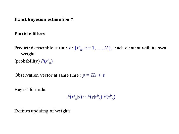
Exact bayesian estimation ? Particle filters Predicted ensemble at time t : {xbn, n = 1, …, N }, each element with its own weight (probability) P(xbn) Observation vector at same time : y = Hx + Bayes’ formula P(xbn y) P(y xbn) P(xbn) Defines updating of weights

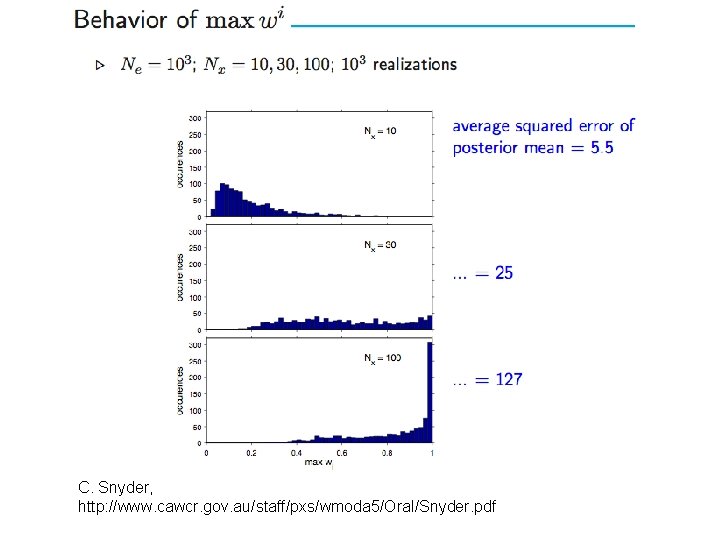
Bayes’ formula P(xbn y) P(y xbn) P(xbn) Defines updating of weights; particles are not modified. Asymptotically converges to bayesian pdf. Very easy to implement. Observed fact. For large state dimension, ensemble tends to collapse.

C. Snyder, http: //www. cawcr. gov. au/staff/pxs/wmoda 5/Oral/Snyder. pdf

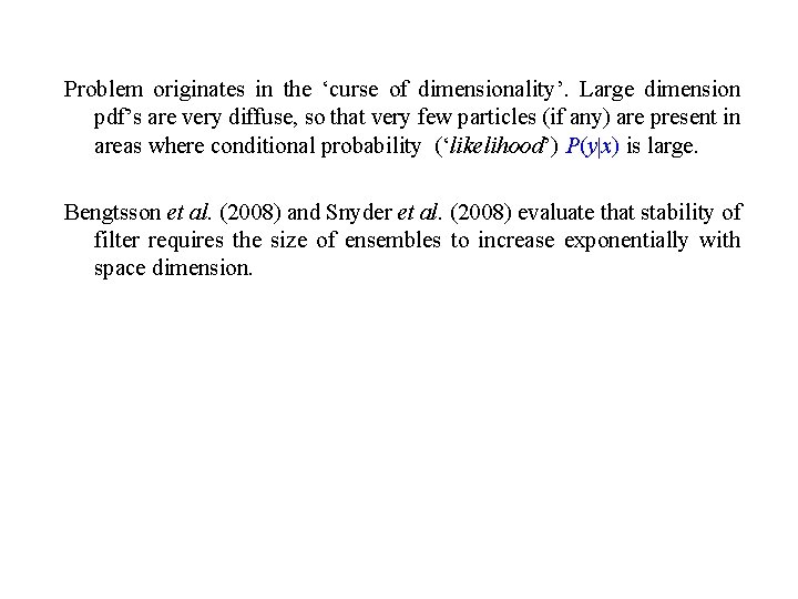
Problem originates in the ‘curse of dimensionality’. Large dimension pdf’s are very diffuse, so that very few particles (if any) are present in areas where conditional probability (‘likelihood’) P(y x) is large. Bengtsson et al. (2008) and Snyder et al. (2008) evaluate that stability of filter requires the size of ensembles to increase exponentially with space dimension.

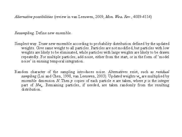
Alternative possibilities (review in van Leeuwen, 2009, Mon. Wea. Rev. , 4089 -4114) Resampling. Define new ensemble. Simplest way. Draw new ensemble according to probability distribution defined by the updated weights. Give same weight to all particles. Particles are not modified, but particles with low weights are likely to be eliminated, while particles with large weights are likely to be drawn repeatedly. For multiple particles, add noise, either from the start, or in the form of ‘model noise’ in ensuing temporal integration. Random character of the sampling introduces noise. Alternatives exist, such as residual sampling (Lui and Chen, 1998, van Leeuwen, 2003). Updated weights wn are multiplied by ensemble dimension N. Then p copies of each particle n are taken, where p is the integer part of Nwn. Remaining particles, if needed, are taken randomly from the resulting distribution.

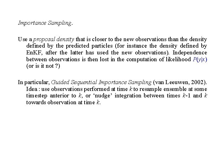
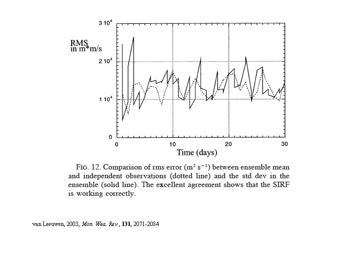
Importance Sampling. Use a proposal density that is closer to the new observations than the density defined by the predicted particles (for instance the density defined by En. KF, after the latter has used the new observations). Independence between observations is then lost in the computation of likelihood P(y x) (or is it not ? ) In particular, Guided Sequential Importance Sampling (van Leeuwen, 2002). Idea : use observations performed at time k to resample ensemble at some timestep anterior to k, or ‘nudge’ integration between times k-1 and k towards observation at time k.

van Leeuwen, 2003, Mon. Wea. Rev. , 131, 2071 -2084

Particle filters are actively studied (van Leeuwen, Morzfeld, …)

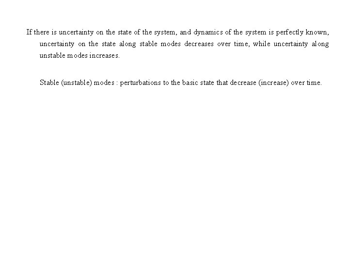
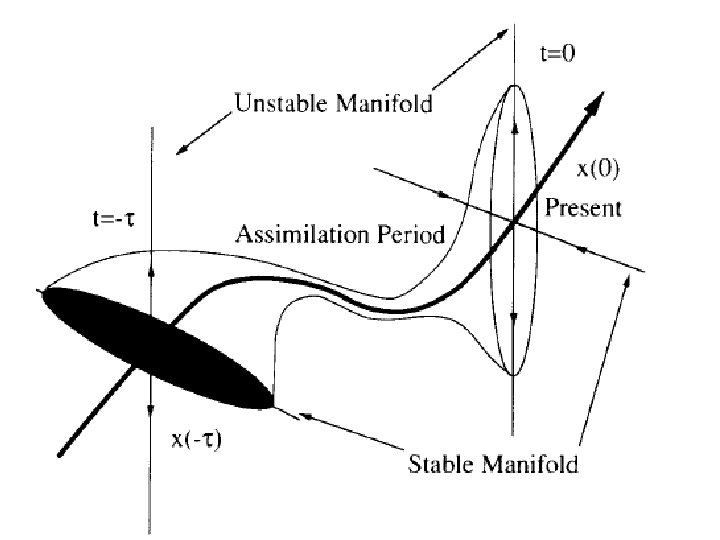
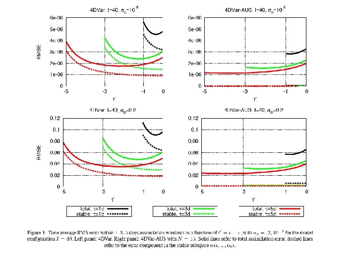
If there is uncertainty on the state of the system, and dynamics of the system is perfectly known, uncertainty on the state along stable modes decreases over time, while uncertainty along unstable modes increases. Stable (unstable) modes : perturbations to the basic state that decrease (increase) over time.

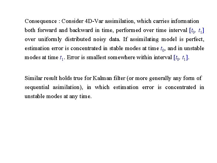
Consequence : Consider 4 D-Var assimilation, which carries information both forward and backward in time, performed over time interval [t 0, t 1] over uniformly distributed noisy data. If assimilating model is perfect, estimation error is concentrated in stable modes at time t 0, and in unstable modes at time t 1. Error is smallest somewhere within interval [t 0, t 1]. Similar result holds true for Kalman filter (or more generally any form of sequential asimilation), in which estimation error is concentrated in unstable modes at any time.

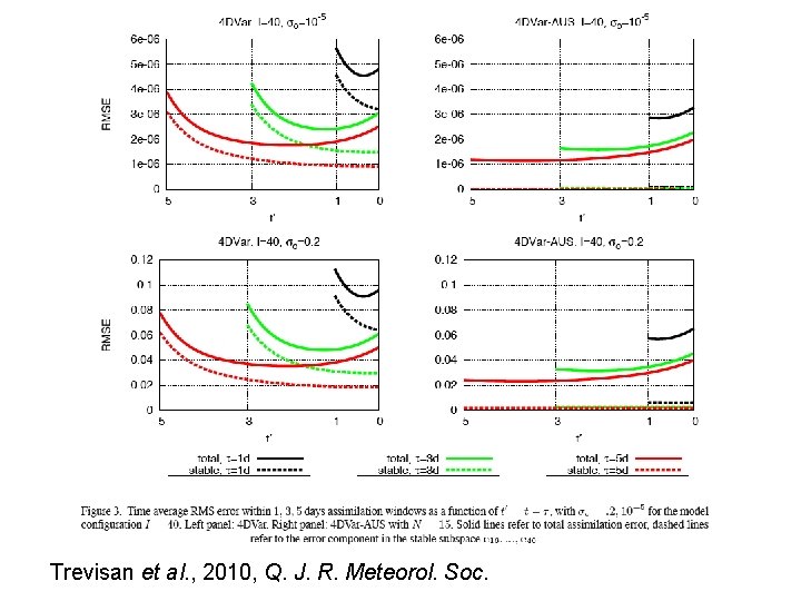
Trevisan et al. , 2010, Q. J. R. Meteorol. Soc.

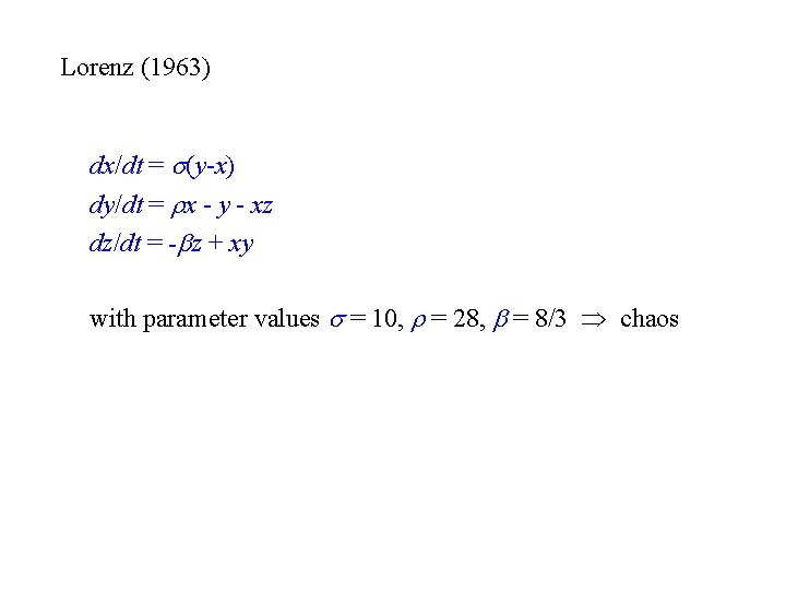
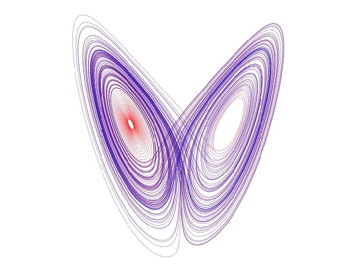
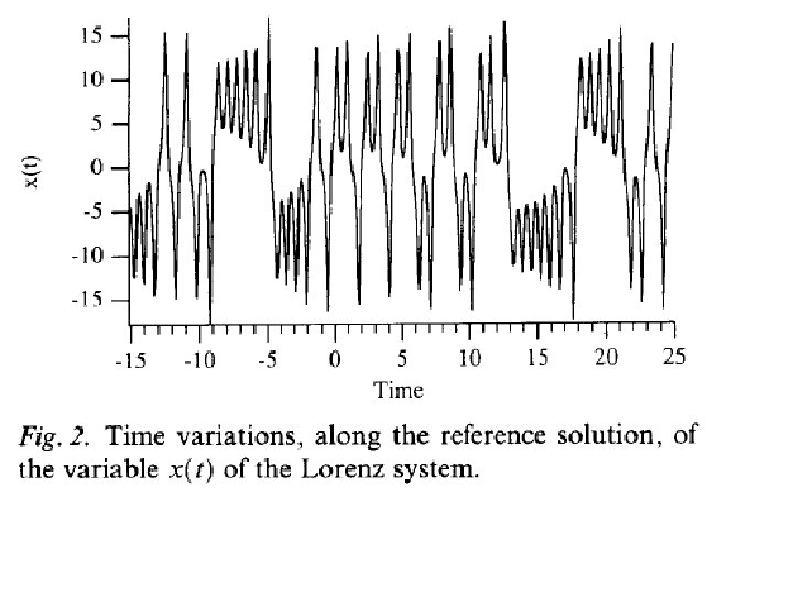
Lorenz (1963) dx/dt = (y-x) dy/dt = x - y - xz dz/dt = - z + xy with parameter values = 10, = 28, = 8/3 chaos

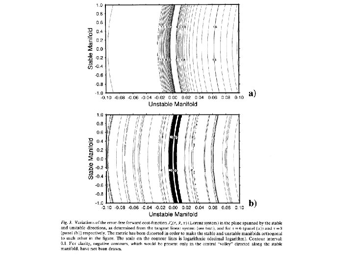
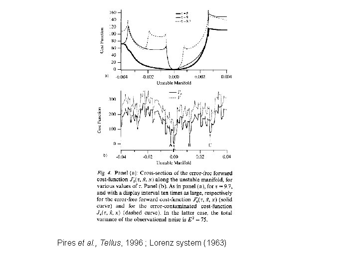
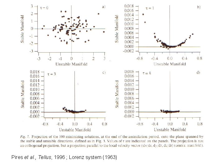
Pires et al. , Tellus, 1996 ; Lorenz system (1963)

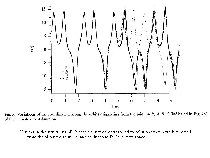
Minima in the variations of objective function correspond to solutions that have bifurcated from the observed solution, and to different folds in state space.

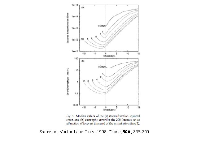
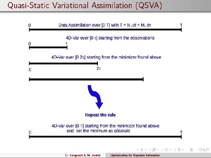
Quasi-Static Variational Assimilation (QSVA). Increase progressively length of the assimilation window, starting each new assimilation from the result of the previous one. This should ensure, at least if observations are in a sense sufficiently dense in time, that current estimation of the system always lies in the attractive basin of the absolute minimum of objective function (Pires et al. , Swanson et al. , Luong, Järvinen et al. ).

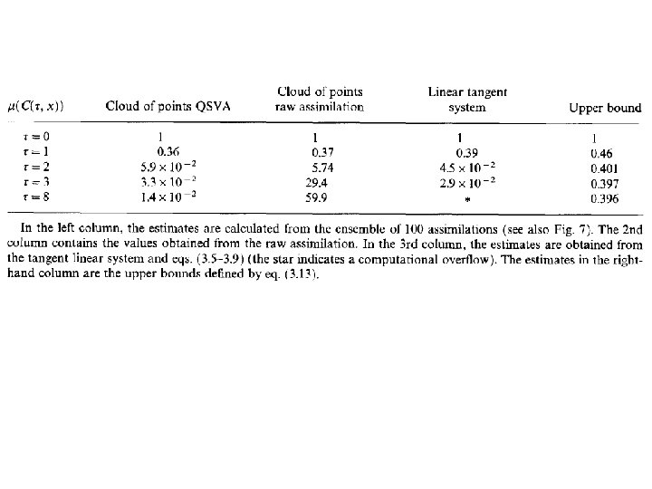
Pires et al. , Tellus, 1996 ; Lorenz system (1963)

Swanson, Vautard and Pires, 1998, Tellus, 50 A, 369 -390

Since, after an assimilation has been performed over a period of time, uncertainty is likely to be concentrated in modes that have been unstable, it might be useful for the next assimilation, and at least in terms of cost efficiency, to concentrate corrections on the background in those modes. Actually, presence of residual noise in stable modes can be damageable for analysis and subsequent forecast. Assimilation in the Unstable Subspace (AUS) (Carrassi et al. , 2007, 2008, for the case of 3 D-Var)

Four-dimensional variational assimilation in the unstable subspace (4 DVar-AUS) Trevisan et al. , 2010, Four-dimensional variational assimilation in the unstable subspace and the optimal subspace dimension, Q. J. R. Meteorol. Soc. , 136, 487 -496.

4 D-Var-AUS Algorithmic implementation Define N perturbations to the current state, and evolve them according to the tangent linear model, with periodic reorthonormalization in order to avoid collapse onto the dominant Lyapunov vector (same algorithm as for computation of Lyapunov exponents). Cycle successive 4 D-Var‘s, restricting at each cycle the modification to be made on the current state to the space spanned by the N perturbations emanating from the previous cycle (if N is the dimension of state space, that is identical with standard 4 D-Var).

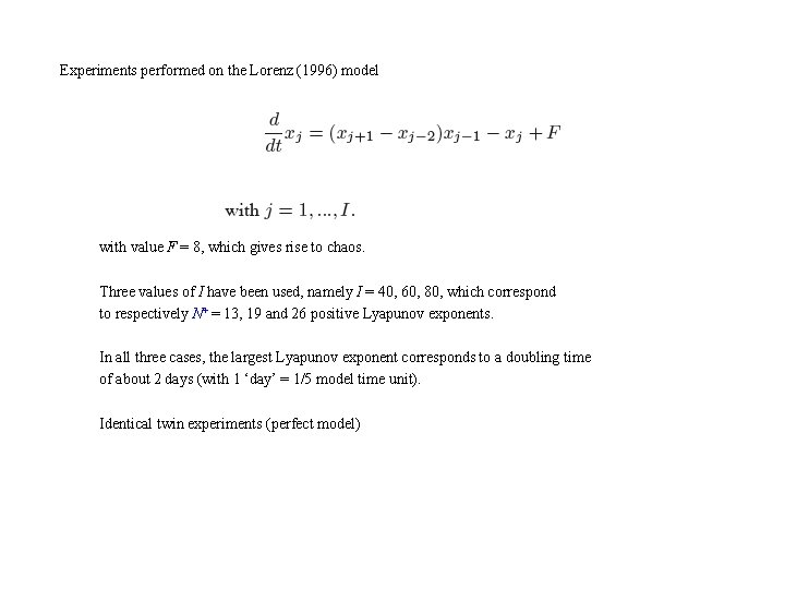
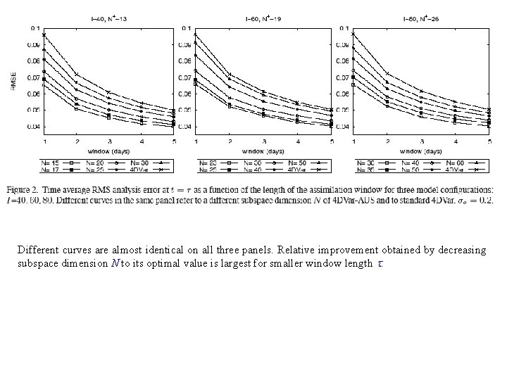
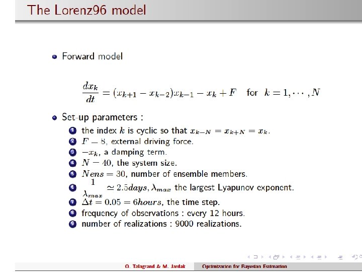
Experiments performed on the Lorenz (1996) model with value F = 8, which gives rise to chaos. Three values of I have been used, namely I = 40, 60, 80, which correspond to respectively N+ = 13, 19 and 26 positive Lyapunov exponents. In all three cases, the largest Lyapunov exponent corresponds to a doubling time of about 2 days (with 1 ‘day’ = 1/5 model time unit). Identical twin experiments (perfect model)

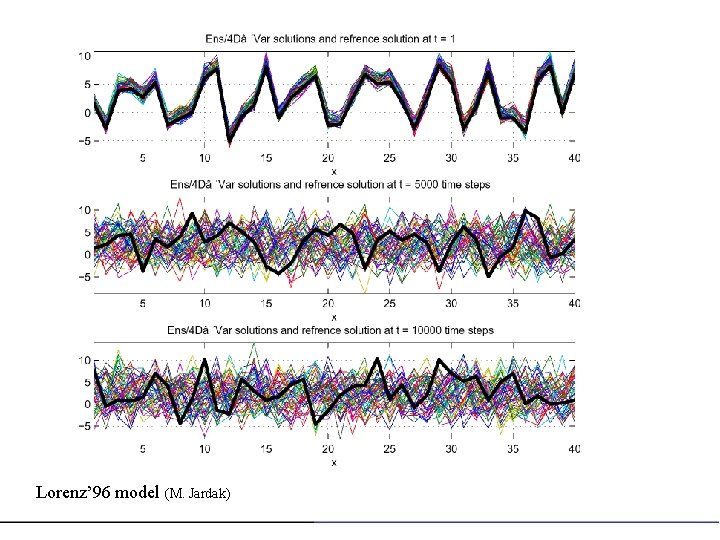
Lorenz’ 96 model (M. Jardak)

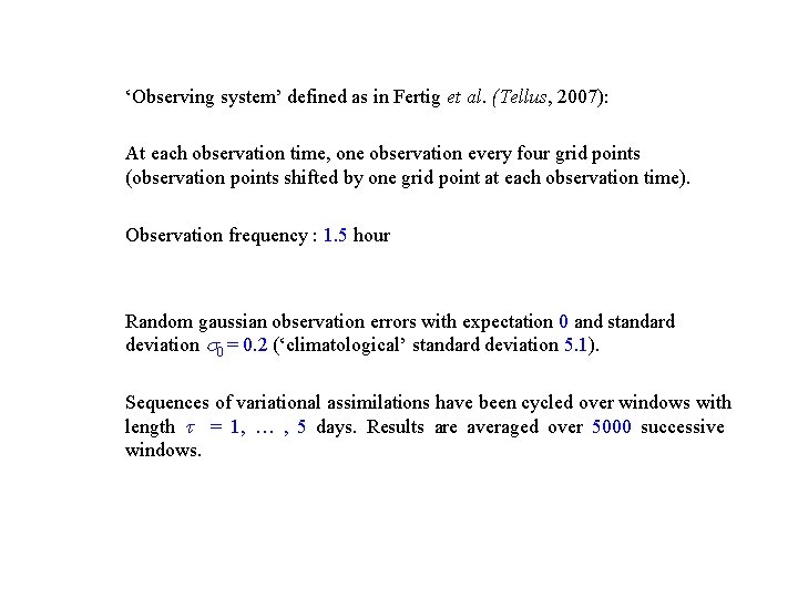
‘Observing system’ defined as in Fertig et al. (Tellus, 2007): At each observation time, one observation every four grid points (observation points shifted by one grid point at each observation time). Observation frequency : 1. 5 hour Random gaussian observation errors with expectation 0 and standard deviation 0 = 0. 2 (‘climatological’ standard deviation 5. 1). Sequences of variational assimilations have been cycled over windows with length = 1, … , 5 days. Results are averaged over 5000 successive windows.

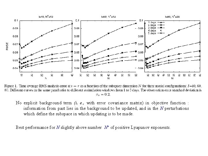
No explicit background term (i. e. , with error covariance matrix) in objective function : information from past lies in the background to be updated, and in the N perturbations which define the subspace in which updating is to be made. Best performance for N slightly above number N+ of positive Lyapunov exponents.

Different curves are almost identical on all three panels. Relative improvement obtained by decreasing subspace dimension N to its optimal value is largest for smaller window length .

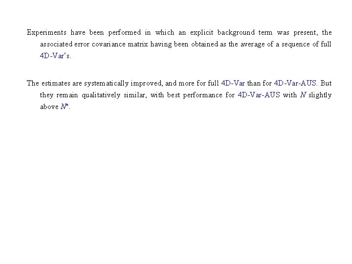
Experiments have been performed in which an explicit background term was present, the associated error covariance matrix having been obtained as the average of a sequence of full 4 D-Var’s. The estimates are systematically improved, and more for full 4 D-Var than for 4 D-Var-AUS. But they remain qualitatively similar, with best performance for 4 D-Var-AUS with N slightly above N+.

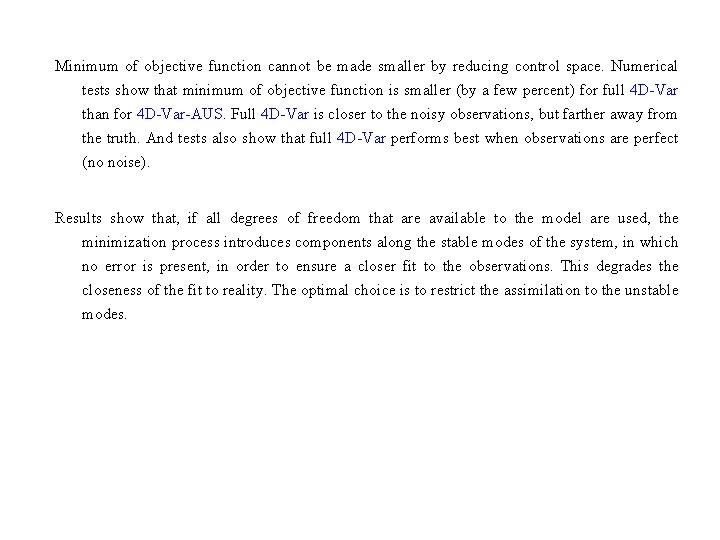
Minimum of objective function cannot be made smaller by reducing control space. Numerical tests show that minimum of objective function is smaller (by a few percent) for full 4 D-Var than for 4 D-Var-AUS. Full 4 D-Var is closer to the noisy observations, but farther away from the truth. And tests also show that full 4 D-Var performs best when observations are perfect (no noise). Results show that, if all degrees of freedom that are available to the model are used, the minimization process introduces components along the stable modes of the system, in which no error is present, in order to ensure a closer fit to the observations. This degrades the closeness of the fit to reality. The optimal choice is to restrict the assimilation to the unstable modes.

Can have major practical algorithmic implications. Questions. - Degree of generality of results ? - Impact of model errors ?

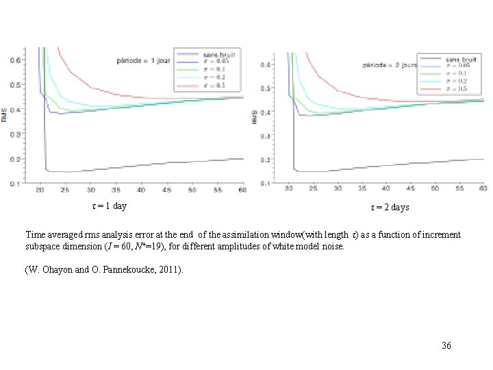
= 1 day = 2 days Time averaged rms analysis error at the end of the assimilation window(with length ) as a function of increment subspace dimension (I = 60, N+=19), for different amplitudes of white model noise. (W. Ohayon and O. Pannekoucke, 2011). 36

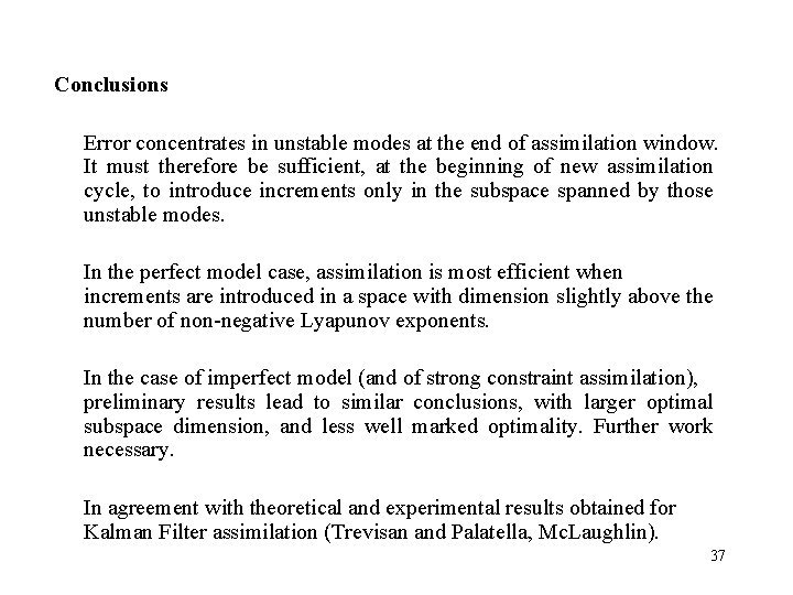
Conclusions Error concentrates in unstable modes at the end of assimilation window. It must therefore be sufficient, at the beginning of new assimilation cycle, to introduce increments only in the subspace spanned by those unstable modes. In the perfect model case, assimilation is most efficient when increments are introduced in a space with dimension slightly above the number of non-negative Lyapunov exponents. In the case of imperfect model (and of strong constraint assimilation), preliminary results lead to similar conclusions, with larger optimal subspace dimension, and less well marked optimality. Further work necessary. In agreement with theoretical and experimental results obtained for Kalman Filter assimilation (Trevisan and Palatella, Mc. Laughlin). 37

Ensemble Variational Assimilation and Bayesian Estimation Olivier Talagrand 1 and Mohamed Jardak 1, 2 1. Laboratoire de Météorologie Dynamique/IPSL École Normale Supérieure, Paris, France 2. Meteorological Office, Exeter, UK Workshop Theoretical aspects of ensemble data assimilation for the Earth system Les Houches, France 6 April 2015 38

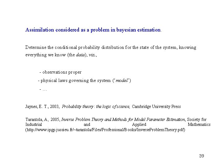
Assimilation considered as a problem in bayesian estimation. Determine the conditional probability distribution for the state of the system, knowing everything we know (the data), viz. , - observations proper - physical laws governing the system (‘model’) -… Jaynes, E. T. , 2003, Probability theory: the logic of science, Cambridge University Press Tarantola, A. , 2005, Inverse Problem Theory and Methods for Model Parameter Estimation, Society for Industrial and Applied Mathematics (http: //www. ipgp. jussieu. fr/~tarantola/Files/Professional/Books/Inverse. Problem. Theory. pdf) 39

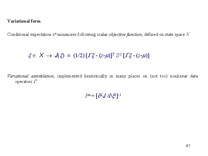
Data of the form z = x + N [ , S] Known data vector z belongs to data space D, dim. D = m, Unknown state vector x belongs to state space X, dim. X = n known (mxn)-matrix, unknown ‘error’ Then conditional probability distribution is P(x z) = N [xa, Pa] where xa = ( T S-1 )-1 T S-1 [z ] Pa = ( T S-1 )-1 Determinacy condition : rank = n. Requires m ≥ n. 40

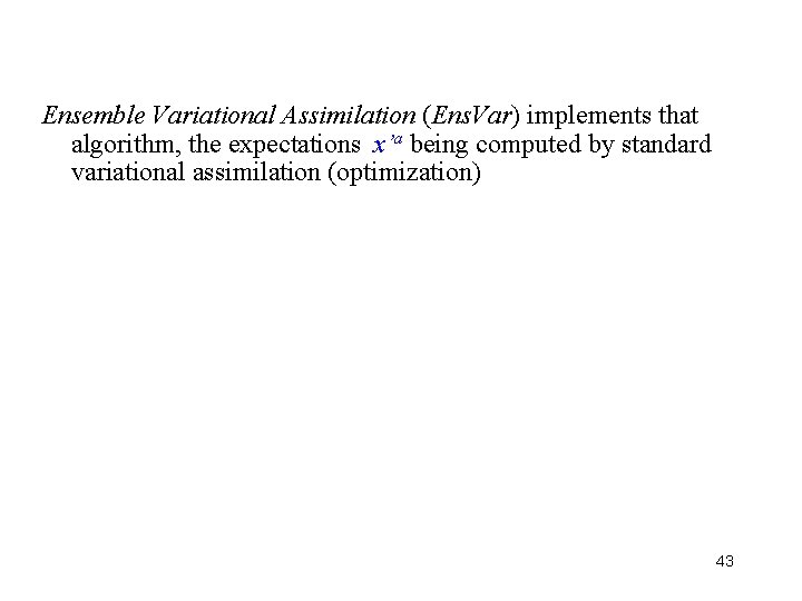
Variational form. Conditional expectation xa minimizes following scalar objective function, defined on state space X X J( ) (1/2) [ - (z- )]T S-1 [ - (z- )] Variational assimilation, implemented heuristically in many places on (not too) nonlinear data operators . Pa = [∂2 J /∂ 2]-1 41

Conditional probability distribution P(x z) = N [xa, Pa] with xa = ( T S-1 )-1 T S-1 [z ] Pa = ( T S-1 )-1 Ready recipe for determining Monte-Carlo sample of conditional pdf P(x z) : - Perturb data vector z according to its own error probability distribution z z’ = z + d d N [0, S] and compute x’a = ( T S-1 )-1 T S-1 [z’ ] x’a is distributed according to N [xa, Pa] 42

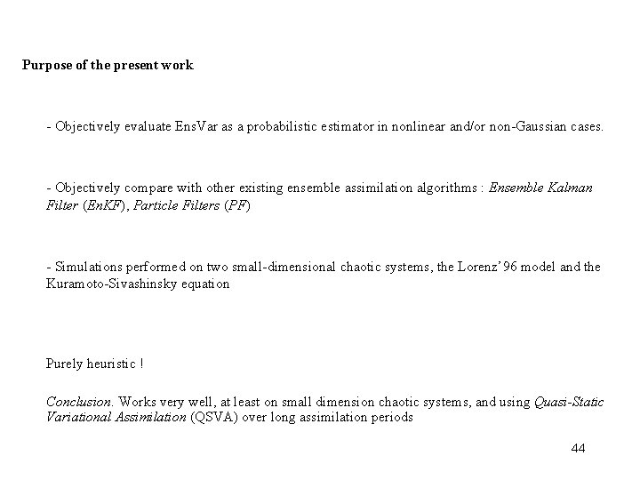
Ensemble Variational Assimilation (Ens. Var) implements that algorithm, the expectations x’a being computed by standard variational assimilation (optimization) 43

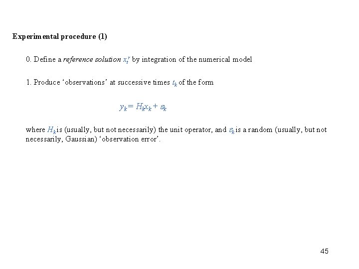
Purpose of the present work - Objectively evaluate Ens. Var as a probabilistic estimator in nonlinear and/or non-Gaussian cases. - Objectively compare with other existing ensemble assimilation algorithms : Ensemble Kalman Filter (En. KF), Particle Filters (PF) - Simulations performed on two small-dimensional chaotic systems, the Lorenz’ 96 model and the Kuramoto-Sivashinsky equation Purely heuristic ! Conclusion. Works very well, at least on small dimension chaotic systems, and using Quasi-Static Variational Assimilation (QSVA) over long assimilation periods 44

Experimental procedure (1) 0. Define a reference solution xtr by integration of the numerical model 1. Produce ‘observations’ at successive times tk of the form yk = Hkxk + k where Hk is (usually, but not necessarily) the unit operator, and k is a random (usually, but not necessarily, Gaussian) ‘observation error’. 45

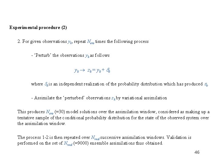
Experimental procedure (2) 2. For given observations yk, repeat Nens times the following process - ‘Perturb’ the observations yk as follows y k zk = y k + dk where dk is an independent realization of the probability distribution which has produced k. - Assimilate the ‘perturbed’ observations zk by variational assimilation This produces Nens (=30) model solutions over the assimilation window, considered as making up a tentative sample of the conditional probability distribution for the state of the observed system over the assimilation window. The process 1 -2 is then repeated over Nreal successive assimilation windows. Validation is performed on the set of Nreal (=9000) ensemble assimilations thus obtained. 46

47

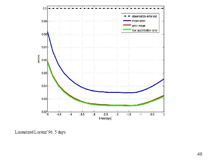
Linearized Lorenz’ 96. 5 days 48

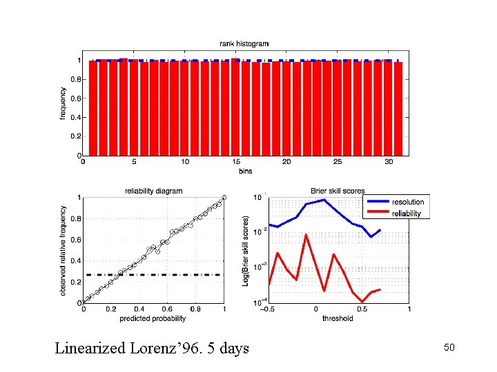
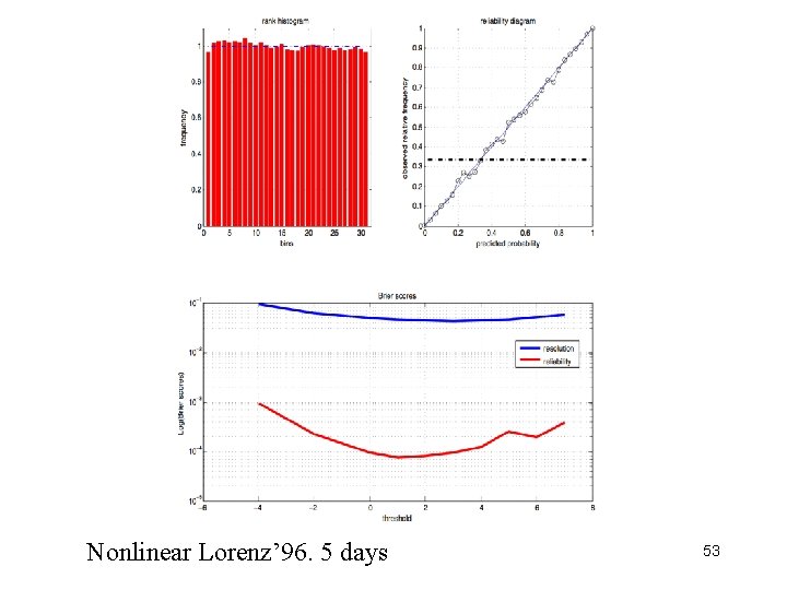
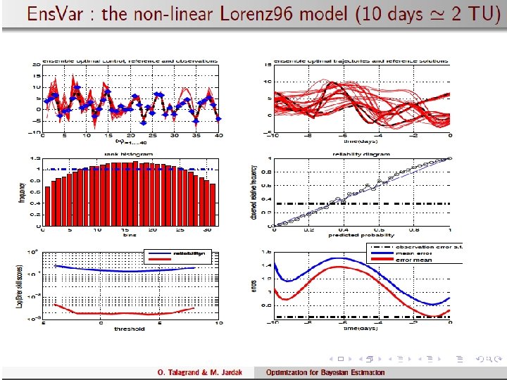
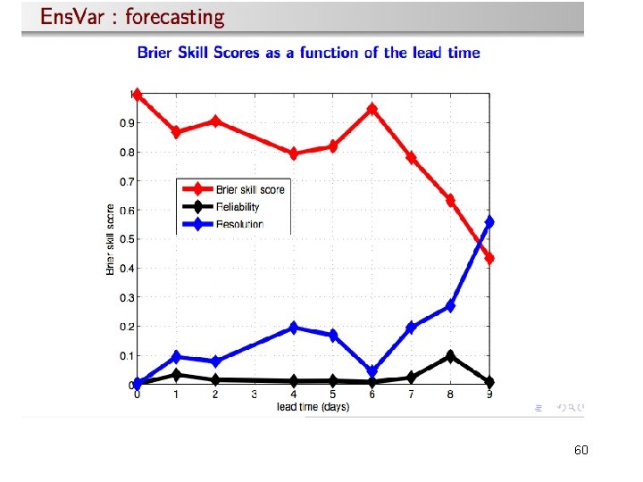
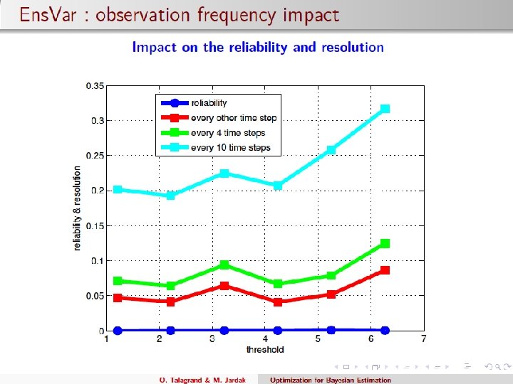
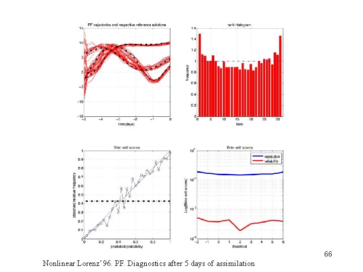
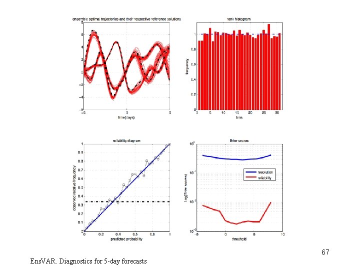
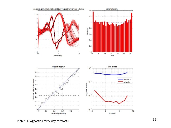
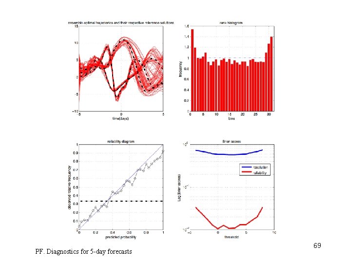
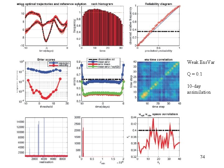
How to objectively evaluate the performance of an ensemble (or more generally probabilistic) estimation system ? - There is no general objective criterion for Bayesianity - We use instead the weaker property of reliability, i. e. statistical consistency between predicted probabilities and observed frequencies of occurrence (it rains with frequency 40% in the circonstances where I have predicted 40% probability for rain). Reliability can be objectively validated, provided a large enough sample of realizations of the estimation system is available. Bayesianity implies reliability, the converse not being true. - We also evaluate resolution, which bears no direct relation to bayesianity, and is best defined as the degree of statistical dependence between the predicted probability distribution and the verifying observation (J. Bröcker). Resolution, beyond reliability, measures the degree of practical accuracy of the ensembles. 49

aaaaa Linearized Lorenz’ 96. 5 days 50

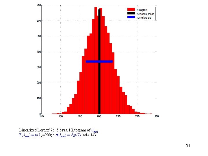
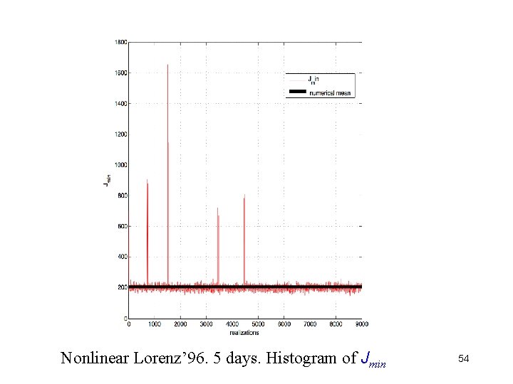
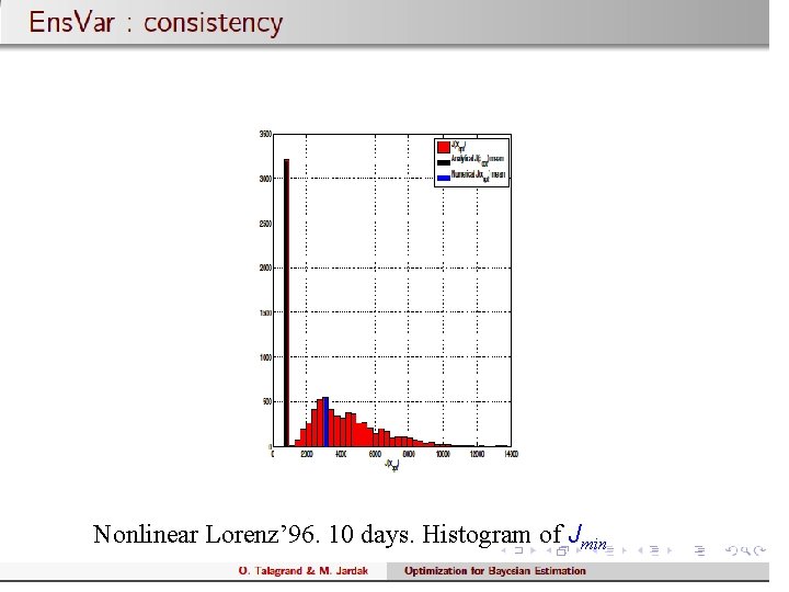
Linearized Lorenz’ 96. 5 days. Histogram of Jmin E(Jmin) = p/2 (=200) ; (Jmin) = √(p/2) (≈14. 14) 51

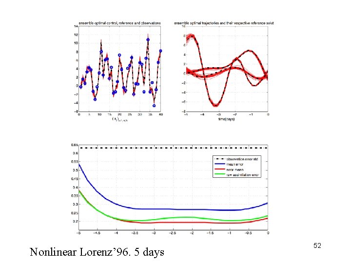
Nonlinear Lorenz’ 96. 5 days 52

Nonlinear Lorenz’ 96. 5 days 53

Nonlinear Lorenz’ 96. 5 days. Histogram of Jmin 54

55

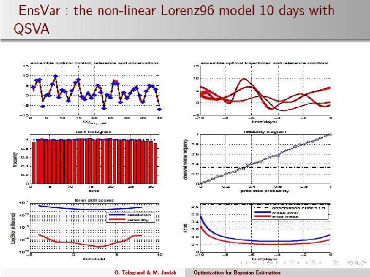
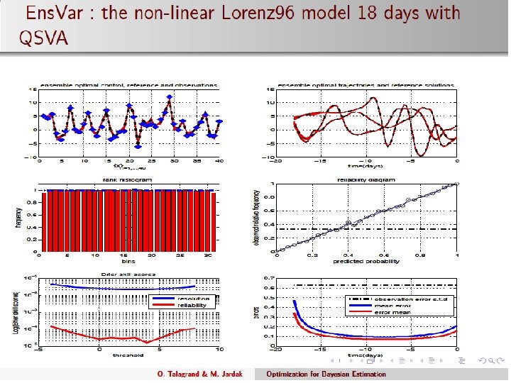
Nonlinear Lorenz’ 96. 10 days. Histogram of Jmin 56

57

58

59

60

61

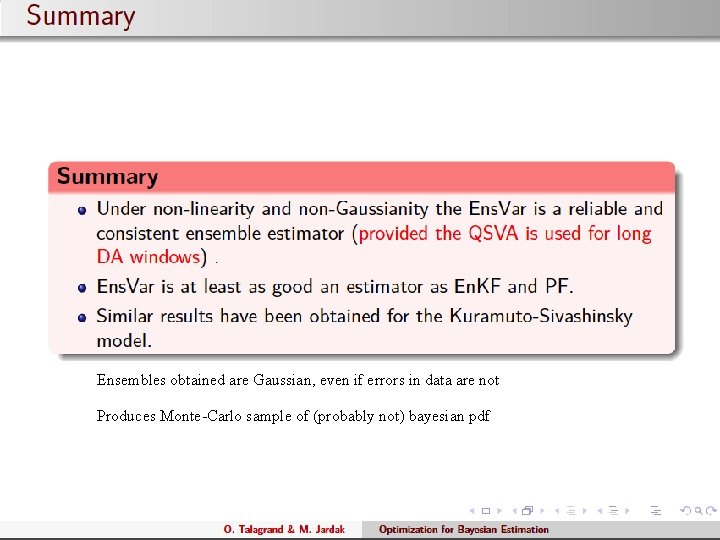
- Results are independent of the Gaussian character of the observation errors (trials have been made with various probability distributions) - Ensembles produced by Ens. Var are very close to Gaussian, even in strongly nonlinear cases. 62

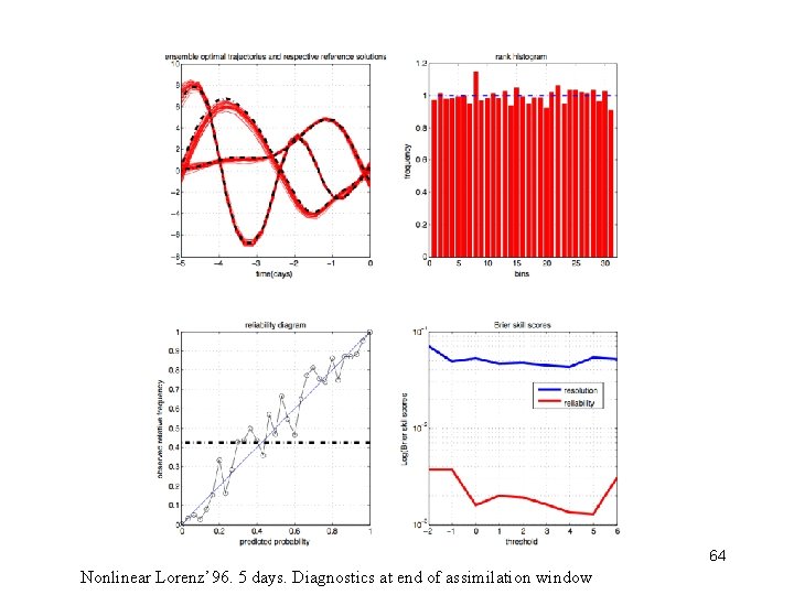
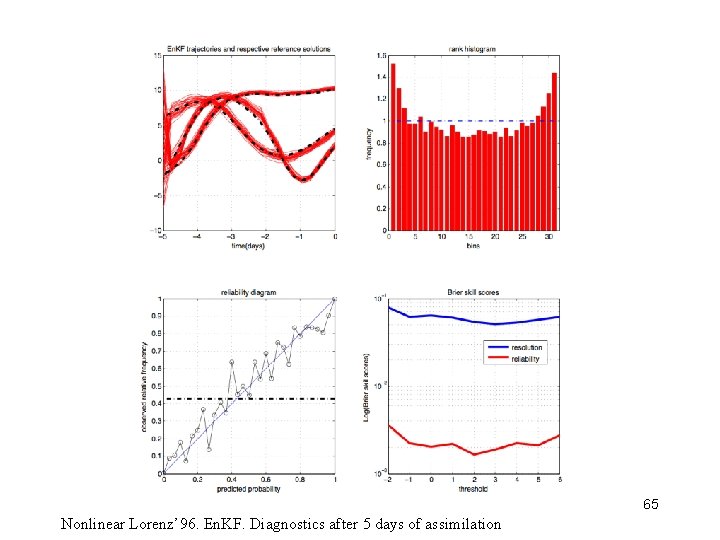
- Comparison Ensemble Kalman Filter (En. KF) and Particle Filters (PF) Both of these algorithms being sequential, comparison is fair only at end of assimilation window 63

64 Nonlinear Lorenz’ 96. 5 days. Diagnostics at end of assimilation window

65 Nonlinear Lorenz’ 96. En. KF. Diagnostics after 5 days of assimilation

66 Nonlinear Lorenz’ 96. PF. Diagnostics after 5 days of assimilation

67 Ens. VAR. Diagnostics for 5 -day forecasts

En. KF. Diagnostics for 5 -day forecasts 68

PF. Diagnostics for 5 -day forecasts 69

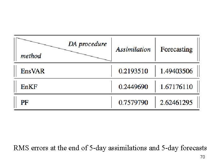
RMS errors at the end of 5 -day assimilations and 5 -day forecasts 70

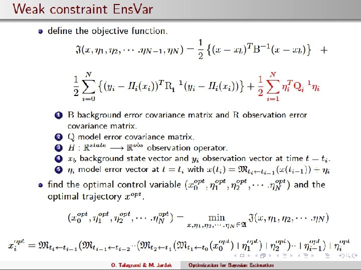
71

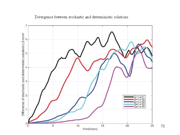
Divergence between stochastic and deterministic solutions 72

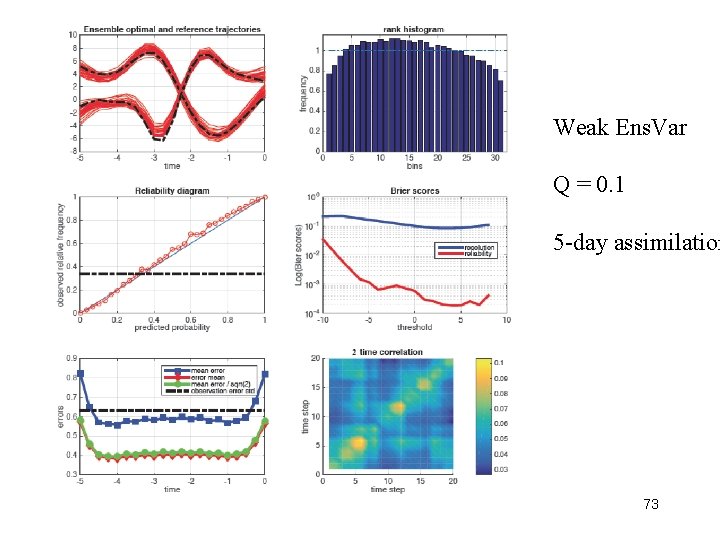
Weak Ens. Var Q = 0. 1 5 -day assimilation 73

Weak Ens. Var Q = 0. 1 10 -day assimilation 74

Ensembles obtained are Gaussian, even if errors in data are not Produces Monte-Carlo sample of (probably not) bayesian pdf 75

76

And now ? - Implementation on physically more realistic models (QG, Shallow water, …) - Comparison with other ensemble algorithms (IEn. KS) - Cycling and/or overlap - Minimisation in unstable space (AUS, Trevisan et al. ) -… 77

The End 78