cole Doctorale des Sciences de lEnvironnement dledeFrance Anne

École Doctorale des Sciences de l'Environnement d’Île-de-France Année 2009 -2010 Modélisation Numérique de l’Écoulement Atmosphérique et Assimilation d'Observations Olivier Talagrand Cours 4 30 Avril 2010

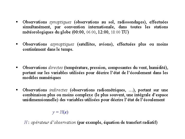
§ Observations synoptiques (observations au sol, radiosondages), effectuées simultanément, par convention internationale, dans toutes les stations météorologiques du globe (00: 00, 06: 00, 12: 00, 18: 00 TU) § Observations asynoptiques (satellites, avions), effectuées plus ou moins continûment dans le temps. § Observations directes (température, pression, composantes du vent, humidité), portant sur les variables utilisées pour décrire l’état de l’écoulement dans les modèles numériques § Observations indirectes (observations radiométriques, …), portant sur une combinaison plus ou moins complexe (le plus souvent, une intégrale d’espace unidimensionnelle) des variables utilisées pour décrire l’état de l’écoulement y = H(x) H : opérateur d’observation (par exemple, équation de transfert radiatif)

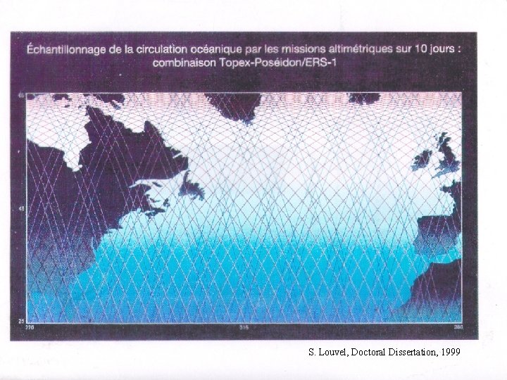
S. Louvel, Doctoral Dissertation, 1999

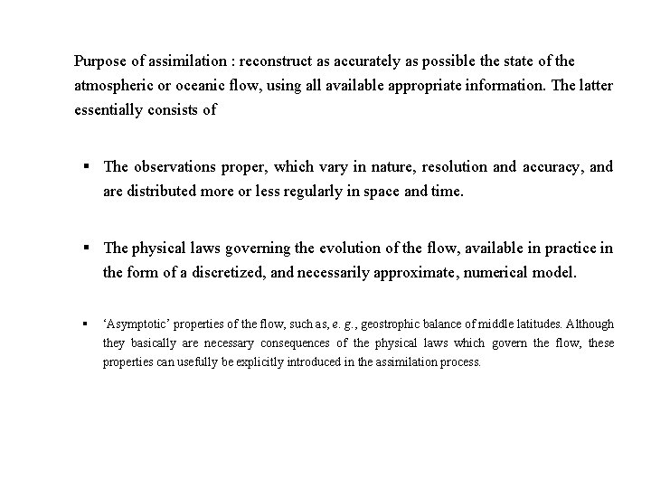
Purpose of assimilation : reconstruct as accurately as possible the state of the atmospheric or oceanic flow, using all available appropriate information. The latter essentially consists of § The observations proper, which vary in nature, resolution and accuracy, and are distributed more or less regularly in space and time. § The physical laws governing the evolution of the flow, available in practice in the form of a discretized, and necessarily approximate, numerical model. § ‘Asymptotic’ properties of the flow, such as, e. g. , geostrophic balance of middle latitudes. Although they basically are necessary consequences of the physical laws which govern the flow, these properties can usefully be explicitly introduced in the assimilation process.

Assimilation is one of many ‘inverse problems’ encountered in many fields of science and technology • solid Earth geophysics • plasma physics • ‘nondestructive’ probing • navigation (spacecraft, aircraft, …. ) • … Solution most often (if not always) based on Bayesian, or probabilistic, estimation. ‘Equations’ are fundamentally the same.

Difficulties specific to assimilation of meteorological observations : - Very large numerical dimensions (n ≈ 106 -109 parameters to be estimated, p ≈ 1 -3. 107 observations per 24 -hour period). Difficulty aggravated in Numerical Weather Prediction by the need for the forecast to be ready in time. - Non-trivial, actually chaotic, underlying dynamics

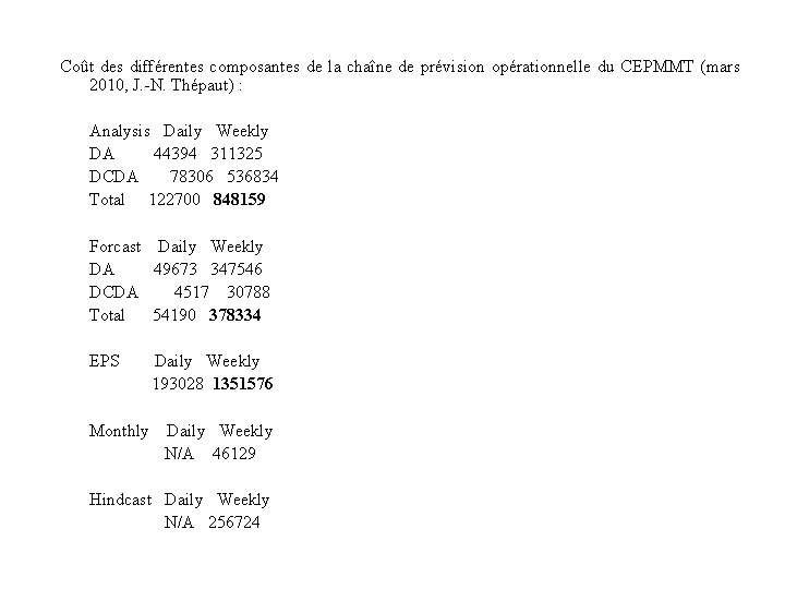
Coût des différentes composantes de la chaîne de prévision opérationnelle du CEPMMT (mars 2010, J. -N. Thépaut) : Analysis Daily Weekly DA 44394 311325 DCDA 78306 536834 Total 122700 848159 Forcast Daily Weekly DA 49673 347546 DCDA 4517 30788 Total 54190 378334 EPS Monthly Daily Weekly 193028 1351576 Daily Weekly N/A 46129 Hindcast Daily Weekly N/A 256724

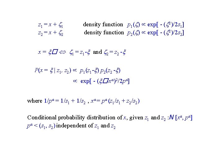
z 1 = x + 1 z 2 = x + 2 density function p 1( ) exp[ - ( 2)/2 s 1] density function p 2( ) exp[ - ( 2)/2 s 2] x = � 1 = z 1 - and 2 = z 2 - P(x = | z 1, z 2) p 1(z 1 - ) p 2(z 2 - ) exp[ - ( �-xa)2/2 pa] where 1/pa = 1/s 1 + 1/s 2 , xa = pa (z 1/s 1 + z 2/s 2) Conditional probability distribution of x, given z 1 and z 2 : N [xa, pa] pa < (s 1, s 2) independent of z 1 and z 2

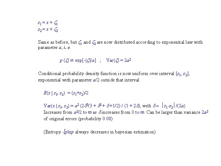
z 1 = x + 1 z 2 = x + 2 Same as before, but 1 and 2 are now distributed according to exponential law with parameter a, i. e. p ( ) exp[-| |/a] ; Var( ) = 2 a 2 Conditional probability density function is now uniform over interval [z 1, z 2], exponential with parameter a/2 outside that interval E(x | z 1, z 2) = (z 1+z 2)/2 Var(x | z 1, z 2) = a 2 (2 3/3 + 2 + +1/2) / (1 + 2 ), with z 1 -z 2 /(2 a) Increases from a 2/2 to as increases from 0 to . Can be larger than variance 2 a 2 of original errors (probability 0. 08) (Entropy - plnp always decreases in bayesian estimation)

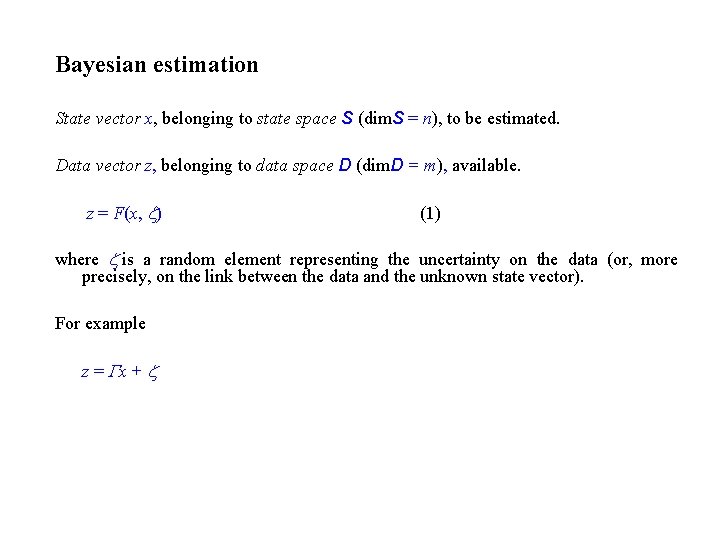
Bayesian estimation State vector x, belonging to state space S (dim. S = n), to be estimated. Data vector z, belonging to data space D (dim. D = m), available. z = F(x, ) (1) where is a random element representing the uncertainty on the data (or, more precisely, on the link between the data and the unknown state vector). For example z = x +

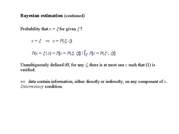
Bayesian estimation (continued) Probability that x = for given ? x = z = F( , ) P(x = | z) = P[z = F( , )] / ’ P[z = F( ’, )] Unambiguously defined iff, for any , there is at most one x such that (1) is verified. data contain information, either directly or indirectly, on any component of x. Determinacy condition.

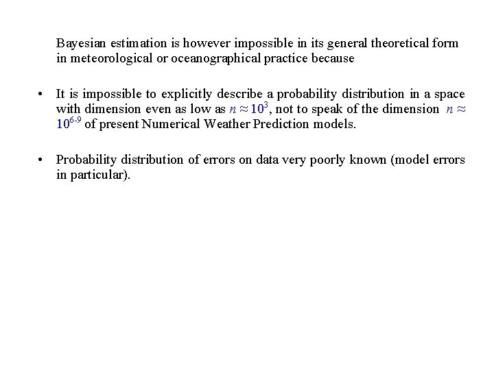
Bayesian estimation is however impossible in its general theoretical form in meteorological or oceanographical practice because • It is impossible to explicitly describe a probability distribution in a space with dimension even as low as n ≈ 103, not to speak of the dimension n ≈ 106 -9 of present Numerical Weather Prediction models. • Probability distribution of errors on data very poorly known (model errors in particular).

One has to restrict oneself to a much more modest goal. Two approaches exist at present § Obtain some ‘central’ estimate of the conditional probability distribution (expectation, mode, …), plus some estimate of the corresponding spread (standard deviations and a number of correlations). § Produce an ensemble of estimates which are meant to sample the conditional probability distribution (dimension N ≈ O(10 -100)).