Chapter 9 Correlation and Regression Elementary Statistics Larson

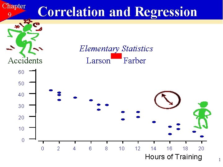
Chapter 9 Correlation and Regression Elementary Statistics Larson Farber Accidents 60 50 40 30 20 10 0 0 2 4 6 8 10 12 14 16 18 20 Hours of Training 1

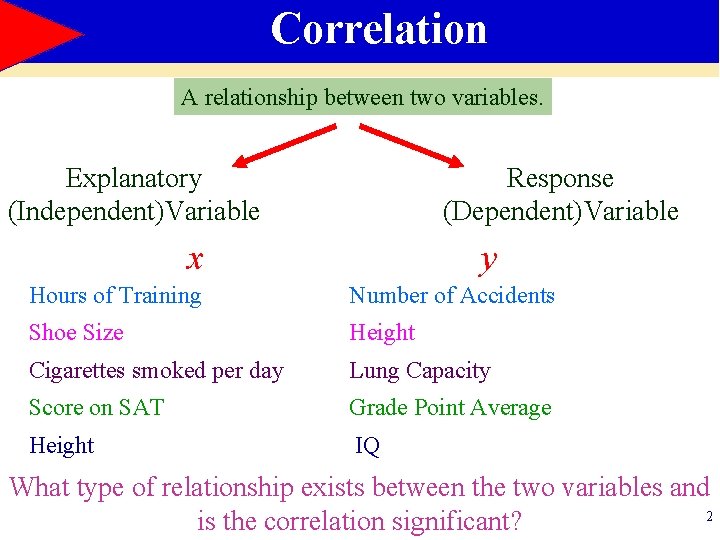
Correlation A relationship between two variables. Explanatory (Independent)Variable Response (Dependent)Variable x y Hours of Training Number of Accidents Shoe Size Height Cigarettes smoked per day Lung Capacity Score on SAT Grade Point Average Height IQ What type of relationship exists between the two variables and 2 is the correlation significant?

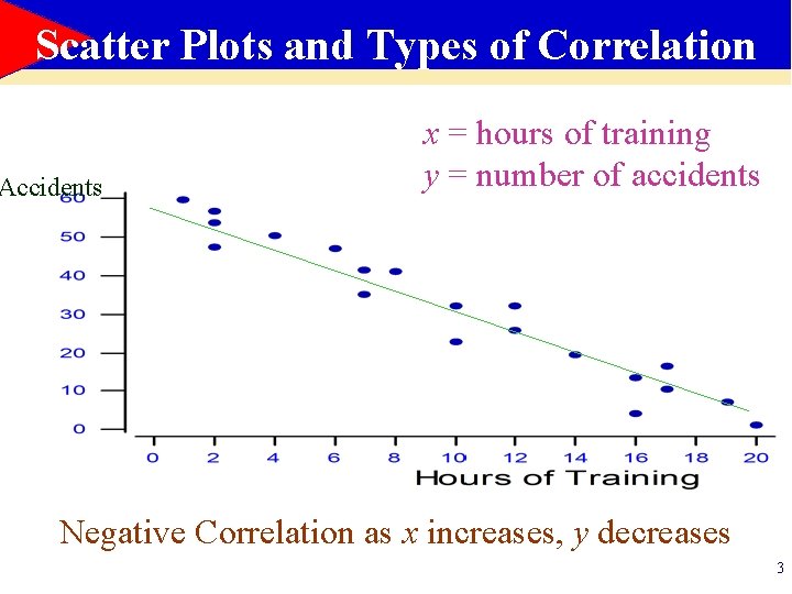
Scatter Plots and Types of Correlation Accidents x = hours of training y = number of accidents Negative Correlation as x increases, y decreases 3

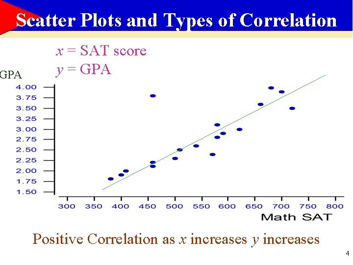
Scatter Plots and Types of Correlation GPA x = SAT score y = GPA Positive Correlation as x increases y increases 4

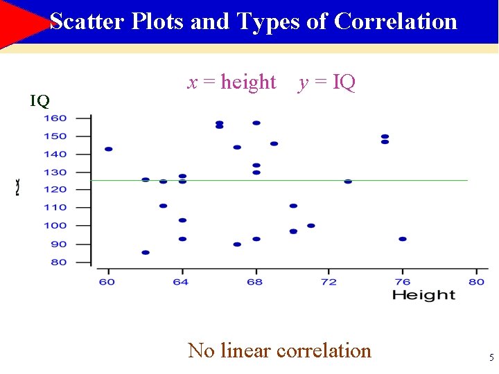
Scatter Plots and Types of Correlation IQ x = height y = IQ No linear correlation 5

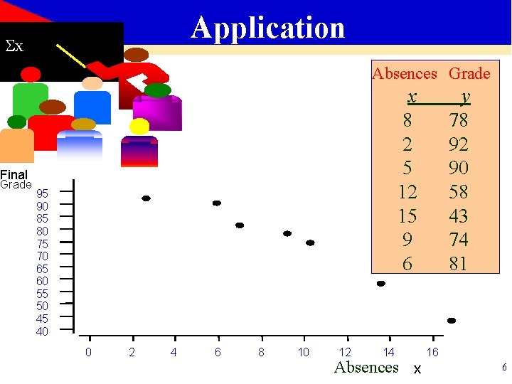
Application x Absences Grade x 8 2 5 12 15 9 6 Final Grade 95 90 85 80 75 70 65 60 55 50 45 40 0 2 4 6 8 10 12 14 Absences x y 78 92 90 58 43 74 81 16 6

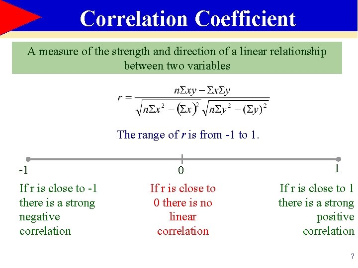
Correlation Coefficient A measure of the strength and direction of a linear relationship between two variables The range of r is from -1 to 1. -1 If r is close to -1 there is a strong negative correlation 0 If r is close to 0 there is no linear correlation 1 If r is close to 1 there is a strong positive correlation 7

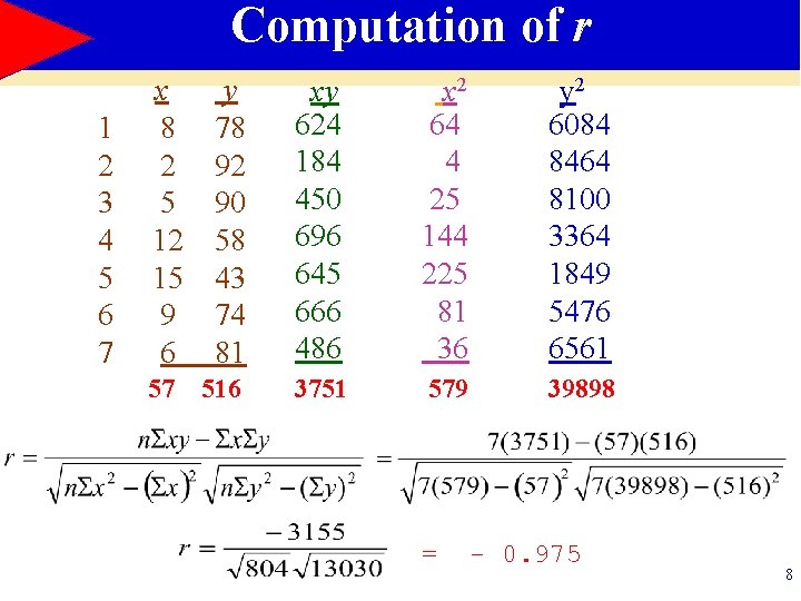
Computation of r 1 2 3 4 5 6 7 x y 8 78 2 92 5 90 12 58 15 43 9 74 6 81 xy 624 184 450 696 645 666 486 x 2 64 4 25 144 225 81 36 y 2 6084 8464 8100 3364 1849 5476 6561 57 3751 579 39898 516 = - 0. 975 8

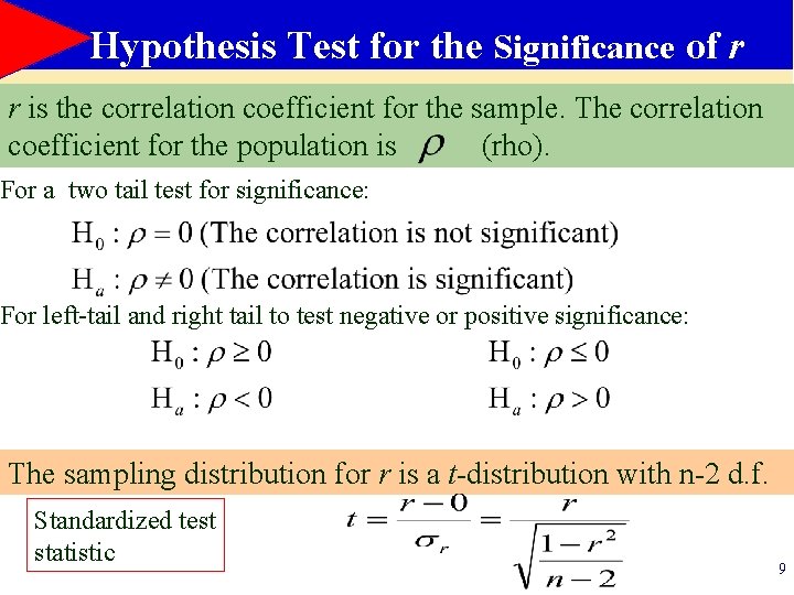
H 0: r = 0 No significant correlation Hypothesis Test for the Significance of r r is the correlation coefficient for the sample. The correlation coefficient for the population is (rho). For a two tail test for significance: For left-tail and right tail to test negative or positive significance: The sampling distribution for r is a t-distribution with n-2 d. f. Standardized test statistic 9

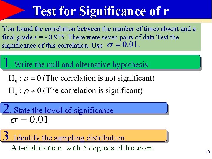
Test for Significance of r You found the correlation between the number of times absent and a final grade r = - 0. 975. There were seven pairs of data. Test the significance of this correlation. Use. 1. Write the null and alternative hypothesis 2. State the level of significance 3. Identify the sampling distribution A t-distribution with 5 degrees of freedom. 10

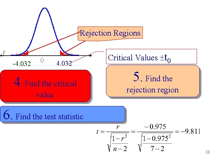
Rejection Regions t -4. 032 0 4. 032 4. Find the critical value Critical Values t 0 5. Find the rejection region 6. Find the test statistic 11

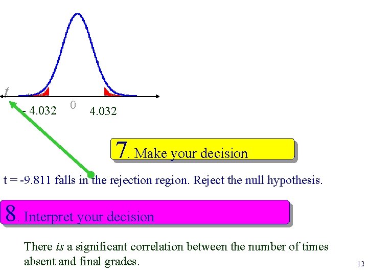
t - 4. 032 0 4. 032 7. Make your decision t = -9. 811 falls in the rejection region. Reject the null hypothesis. 8. Interpret your decision There is a significant correlation between the number of times absent and final grades. 12

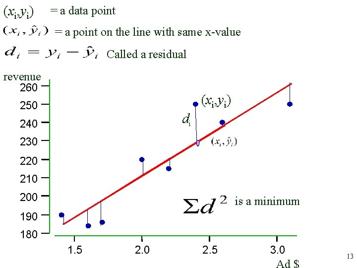
(xi, yi) = a data point = a point on the line with same x-value Called a residual revenue 260 (xi, yi) 250 di 240 230 220 210 200 is a minimum 190 180 1. 5 2. 0 2. 5 3. 0 Ad $ 13

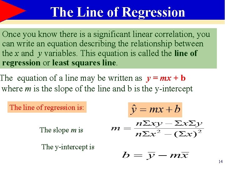
The Line of Regression Once you know there is a significant linear correlation, you can write an equation describing the relationship between the x and y variables. This equation is called the line of regression or least squares line. The equation of a line may be written as y = mx + b where m is the slope of the line and b is the y-intercept The line of regression is: The slope m is The y-intercept is 14

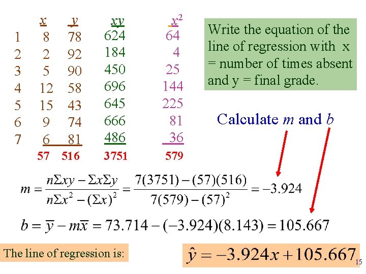
1 2 3 4 5 6 7 x y 8 78 2 92 5 90 12 58 15 43 9 74 6 81 xy 624 184 450 696 645 666 486 x 2 64 4 25 144 225 81 36 57 3751 579 516 The line of regression is: Write the equation of the line of regression with x = number of times absent and y = final grade. Calculate m and b 15

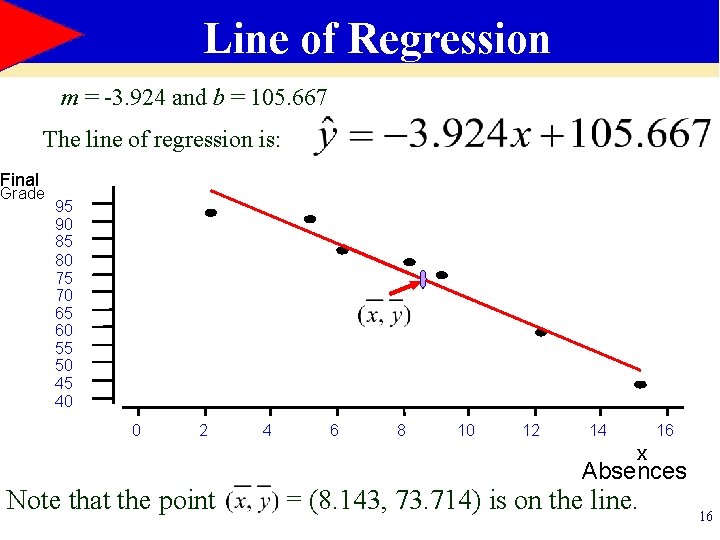
Line of Regression m = -3. 924 and b = 105. 667 The line of regression is: Final Grade 95 90 85 80 75 70 65 60 55 50 45 40 0 2 4 6 8 10 12 14 16 x Note that the point Absences = (8. 143, 73. 714) is on the line. 16

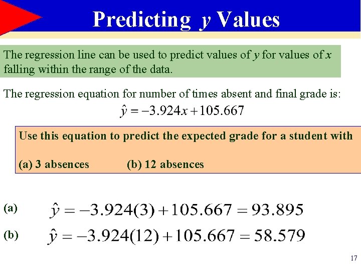
Predicting y Values The regression line can be used to predict values of y for values of x falling within the range of the data. The regression equation for number of times absent and final grade is: Use this equation to predict the expected grade for a student with (a) 3 absences (b) 12 absences (a) (b) 17

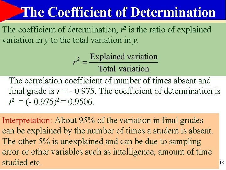
The Coefficient of Determination The coefficient of determination, r 2 is the ratio of explained variation in y to the total variation in y. The correlation coefficient of number of times absent and final grade is r = - 0. 975. The coefficient of determination is r 2 = (- 0. 975)2 = 0. 9506. Interpretation: About 95% of the variation in final grades can be explained by the number of times a student is absent. The other 5% is unexplained and can be due to sampling error or other variables such as intelligence, amount of time studied etc. 18

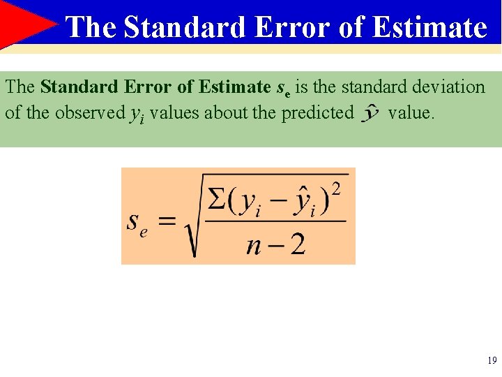
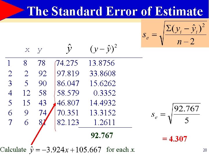
The Standard Error of Estimate se is the standard deviation of the observed yi values about the predicted value. 19

The Standard Error of Estimate x y 1 2 3 4 5 6 7 8 78 2 92 5 90 12 58 15 43 9 74 6 81 Calculate 74. 275 97. 819 86. 047 58. 579 46. 807 70. 351 82. 123 13. 8756 33. 8608 15. 6262 0. 3352 14. 4932 13. 3152 1. 2611 92. 767 for each x. = 4. 307 20

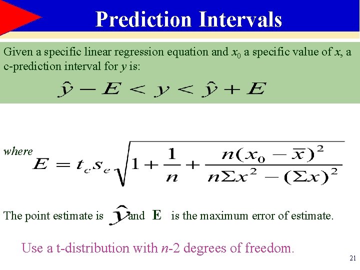
Prediction Intervals Given a specific linear regression equation and x 0 a specific value of x, a c-prediction interval for y is: where The point estimate is and E is the maximum error of estimate. Use a t-distribution with n-2 degrees of freedom. 21

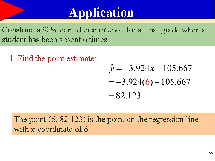
Application Construct a 90% confidence interval for a final grade when a student has been absent 6 times. 1. Find the point estimate: The point (6, 82. 123) is the point on the regression line with x-coordinate of 6. 22

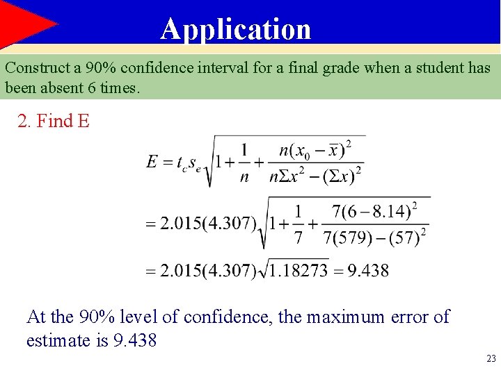
Application Construct a 90% confidence interval for a final grade when a student has been absent 6 times. 2. Find E At the 90% level of confidence, the maximum error of estimate is 9. 438 23

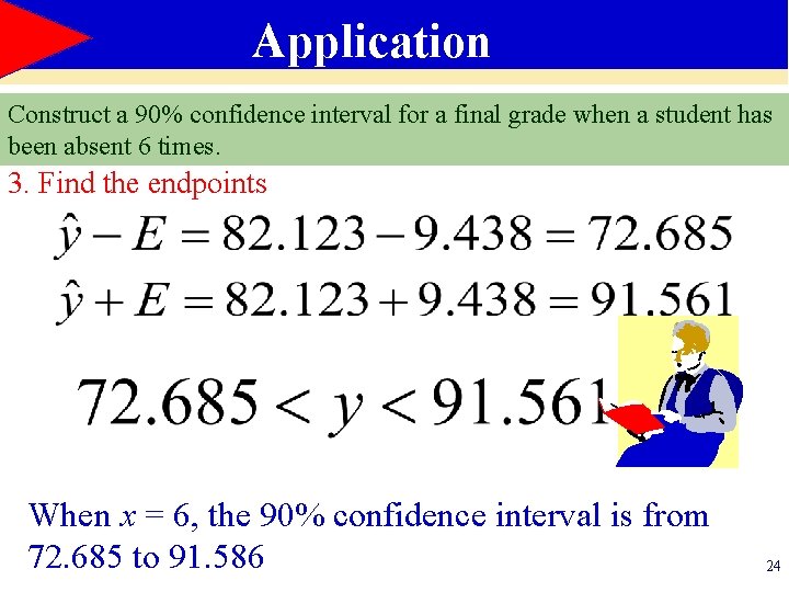
Application Construct a 90% confidence interval for a final grade when a student has been absent 6 times. 3. Find the endpoints When x = 6, the 90% confidence interval is from 72. 685 to 91. 586 24

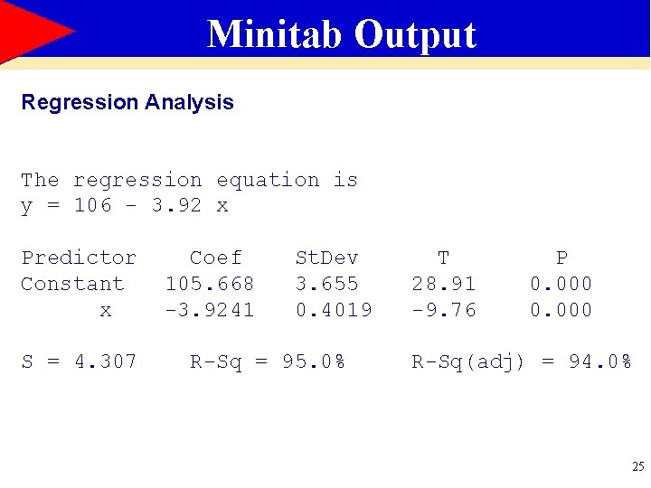
Minitab Output Regression Analysis The regression equation is y = 106 - 3. 92 x Predictor Constant x S = 4. 307 Coef 105. 668 -3. 9241 St. Dev 3. 655 0. 4019 R-Sq = 95. 0% T 28. 91 -9. 76 P 0. 000 R-Sq(adj) = 94. 0% 25