CHAPTER 6 Efficient Diversification The Goals of Chapter

CHAPTER 6 Efficient Diversification

The Goals of Chapter 6 Introduce the market risk (市場風險) and the firm-specific risk (公司特定風險) Portfolio Theory (投資組合理論): – Diversification in the case of two risky assets without or with the risk-free asset – Extension to the multiple risky-asset case Introduce the single-factor model (單一指數模 型), which is a statistical model – To identify the components of firm-specific and market risks – To develop the Treynor-Black model to construct portfolios with higher Sharpe ratios – To examine the CAPM (discussed in Ch 7) 6 -2

6. 1 DIVERSIFICATION AND PORTFOLIO RISK 6 -3

Diversification and Portfolio Risk Firm-specific risk (公司特定風險) – Risk factors that affect an individual firm without noticeably affecting other firms, like the results of R&D, the management style, etc. – Due to the possible offset of the firm-specific risks from different firms in a portfolio, this risk can be eliminated through diversification – Also called unique, idiosyncratic (特質的), diversifiable, or nonsystematic risk Market risk (市場風險) – Risk factors common to the whole economy, possibly from business cycles, inflation rates, interest rates, exchange rates, etc. – The risk cannot be eliminated through diversification – Also called nondiversifiable or systematic risk 6 -4

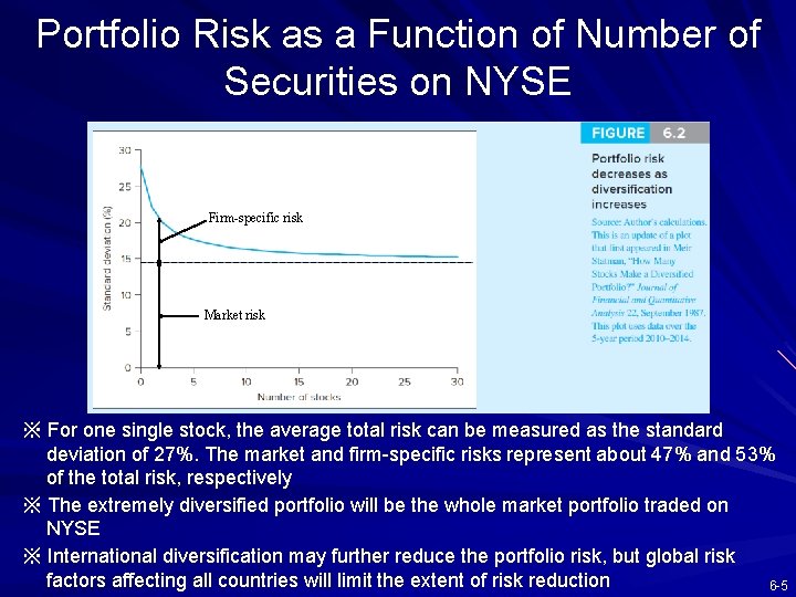
Portfolio Risk as a Function of Number of Securities on NYSE Firm-specific risk Market risk ※ For one single stock, the average total risk can be measured as the standard deviation of 27%. The market and firm-specific risks represent about 47% and 53% of the total risk, respectively ※ The extremely diversified portfolio will be the whole market portfolio traded on NYSE ※ International diversification may further reduce the portfolio risk, but global risk factors affecting all countries will limit the extent of risk reduction 6 -5

6. 2 ASSET ALLOCATION WITH TWO RISKY ASSETS 6 -6

Diversification and Portfolio Theory The portfolio theory was first introduced by Harry Markowitz in 1952, who is a Nobel Prize laureate in 1990 Sections 6. 2 to 6. 4 will introduce the results of Markowitz’s work of showing how to make the most of the power of diversification In this section, the effect of diversification is illustrated by a case of two risky assets 6 -7

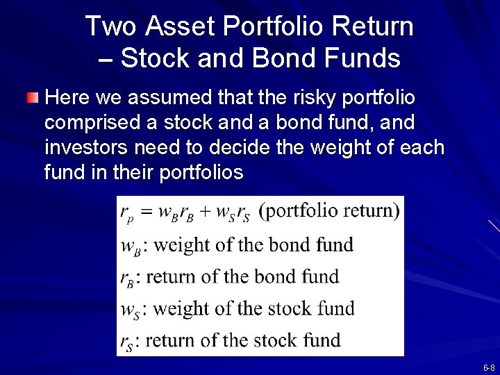
Two Asset Portfolio Return – Stock and Bond Funds Here we assumed that the risky portfolio comprised a stock and a bond fund, and investors need to decide the weight of each fund in their portfolios 6 -8

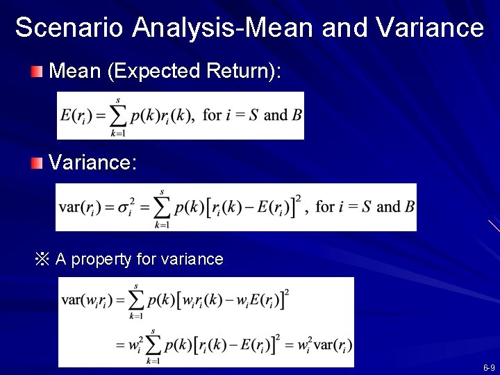
Scenario Analysis-Mean and Variance Mean (Expected Return): Variance: ※ A property for variance 6 -9

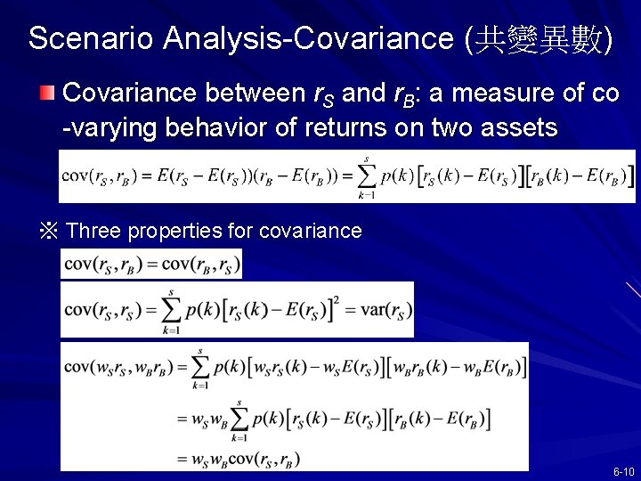
Scenario Analysis-Covariance (共變異數) Covariance between r. S and r. B: a measure of co -varying behavior of returns on two assets ※ Three properties for covariance 6 -10

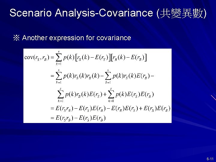
Scenario Analysis-Covariance (共變異數) ※ Another expression for covariance 6 -11

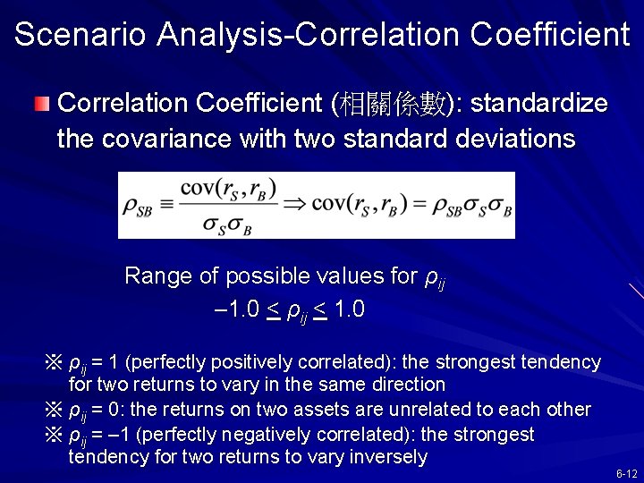
Scenario Analysis-Correlation Coefficient (相關係數): standardize the covariance with two standard deviations Range of possible values for ρij – 1. 0 < ρij < 1. 0 ※ ρij = 1 (perfectly positively correlated): the strongest tendency for two returns to vary in the same direction ※ ρij = 0: the returns on two assets are unrelated to each other ※ ρij = – 1 (perfectly negatively correlated): the strongest tendency for two returns to vary inversely 6 -12

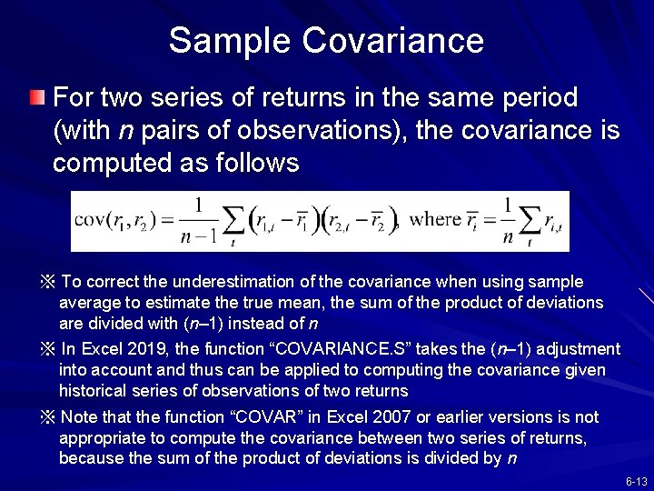
Sample Covariance For two series of returns in the same period (with n pairs of observations), the covariance is computed as follows ※ To correct the underestimation of the covariance when using sample average to estimate the true mean, the sum of the product of deviations are divided with (n– 1) instead of n ※ In Excel 2019, the function “COVARIANCE. S” takes the (n– 1) adjustment into account and thus can be applied to computing the covariance given historical series of observations of two returns ※ Note that the function “COVAR” in Excel 2007 or earlier versions is not appropriate to compute the covariance between two series of returns, because the sum of the product of deviations is divided by n 6 -13

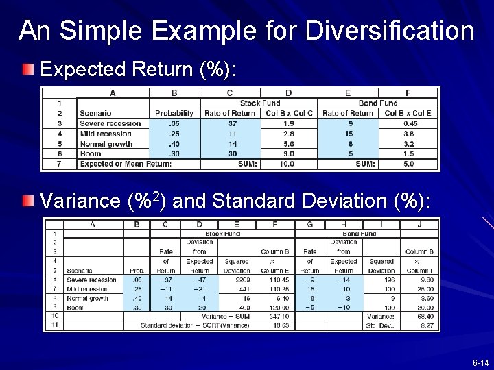
An Simple Example for Diversification Expected Return (%): Variance (%2) and Standard Deviation (%): 6 -14

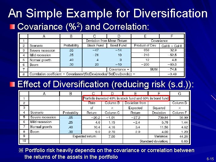
An Simple Example for Diversification Covariance (%2) and Correlation: Effect of Diversification (reducing risk (s. d. )): ※ Portfolio risk heavily depends on the covariance or correlation between the returns of the assets in the portfolio 6 -15

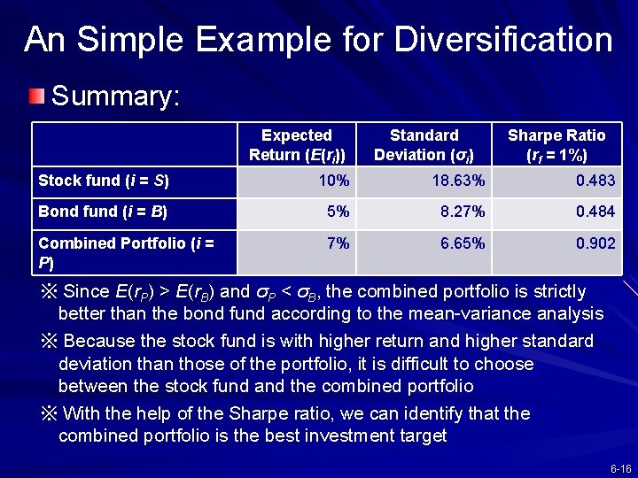
An Simple Example for Diversification Summary: Expected Return (E(ri)) Standard Deviation (σi) Sharpe Ratio (rf = 1%) Stock fund (i = S) 10% 18. 63% 0. 483 Bond fund (i = B) 5% 8. 27% 0. 484 Combined Portfolio (i = P) 7% 6. 65% 0. 902 ※ Since E(r. P) > E(r. B) and σP < σB, the combined portfolio is strictly better than the bond fund according to the mean-variance analysis ※ Because the stock fund is with higher return and higher standard deviation than those of the portfolio, it is difficult to choose between the stock fund and the combined portfolio ※ With the help of the Sharpe ratio, we can identify that the combined portfolio is the best investment target 6 -16

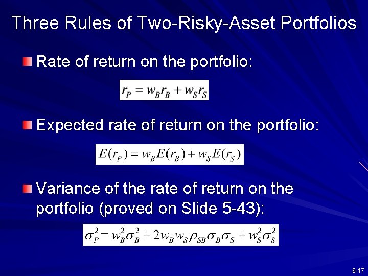
Three Rules of Two-Risky-Asset Portfolios Rate of return on the portfolio: Expected rate of return on the portfolio: Variance of the rate of return on the portfolio (proved on Slide 5 -43): 6 -17

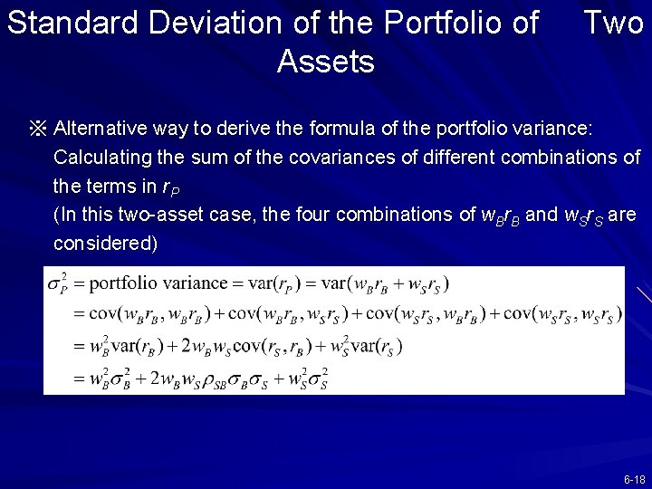
Standard Deviation of the Portfolio of Assets Two ※ Alternative way to derive the formula of the portfolio variance: Calculating the sum of the covariances of different combinations of the terms in r. P (In this two-asset case, the four combinations of w. Br. B and w. Sr. S are considered) 6 -18

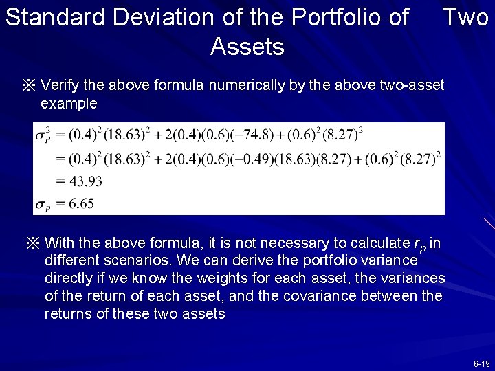
Standard Deviation of the Portfolio of Assets Two ※ Verify the above formula numerically by the above two-asset example ※ With the above formula, it is not necessary to calculate rp in different scenarios. We can derive the portfolio variance directly if we know the weights for each asset, the variances of the return of each asset, and the covariance between the returns of these two assets 6 -19

Three Rules for an n-Security Portfolio: 6 -20

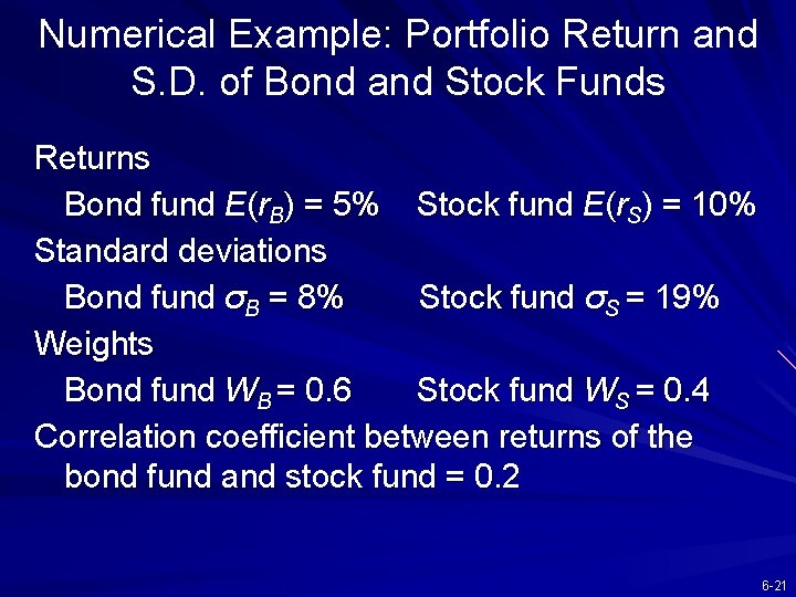
Numerical Example: Portfolio Return and S. D. of Bond and Stock Funds Returns Bond fund E(r. B) = 5% Stock fund E(r. S) = 10% Standard deviations Bond fund σB = 8% Stock fund σS = 19% Weights Bond fund WB = 0. 6 Stock fund WS = 0. 4 Correlation coefficient between returns of the bond fund and stock fund = 0. 2 6 -21

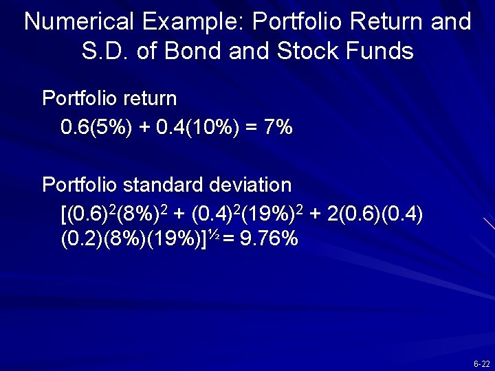
Numerical Example: Portfolio Return and S. D. of Bond and Stock Funds Portfolio return 0. 6(5%) + 0. 4(10%) = 7% Portfolio standard deviation [(0. 6)2(8%)2 + (0. 4)2(19%)2 + 2(0. 6)(0. 4) (0. 2)(8%)(19%)]½ = 9. 76% 6 -22

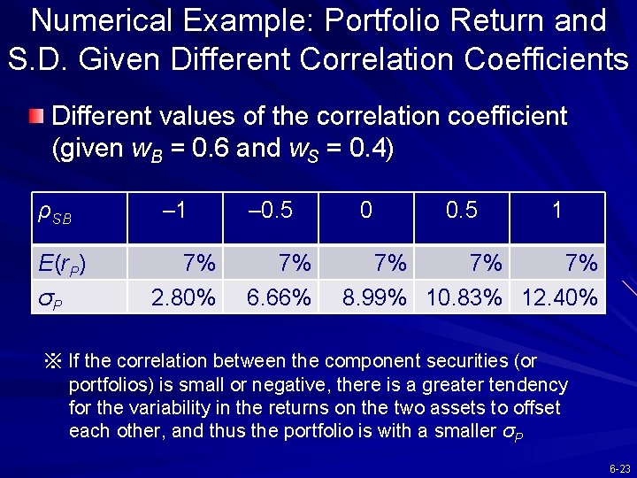
Numerical Example: Portfolio Return and S. D. Given Different Correlation Coefficients Different values of the correlation coefficient (given w. B = 0. 6 and w. S = 0. 4) ρSB E(r. P) σP – 1 7% 2. 80% – 0. 5 7% 6. 66% 0 0. 5 1 7% 7% 7% 8. 99% 10. 83% 12. 40% ※ If the correlation between the component securities (or portfolios) is small or negative, there is a greater tendency for the variability in the returns on the two assets to offset each other, and thus the portfolio is with a smaller σP 6 -23

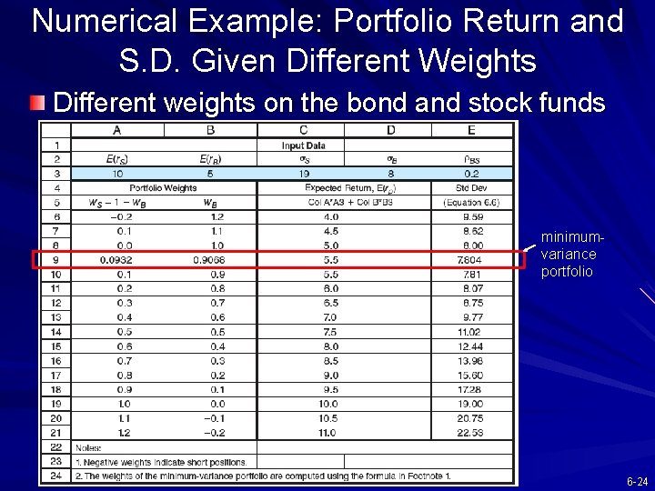
Numerical Example: Portfolio Return and S. D. Given Different Weights Different weights on the bond and stock funds minimumvariance portfolio 6 -24

Numerical Example: Portfolio Return of Bond and Stock Funds (Page 155) The weights for the minimum-variance portfolio 6 -25

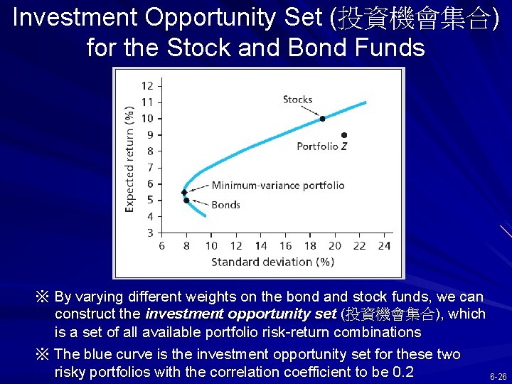
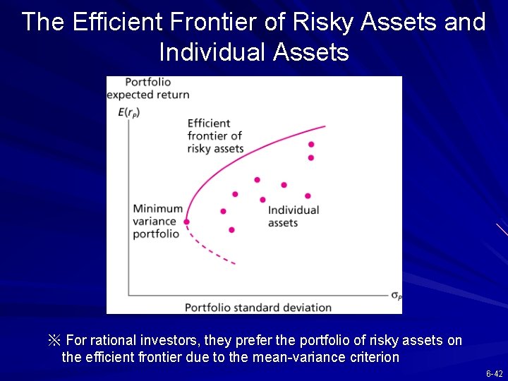
Investment Opportunity Set (投資機會集合) for the Stock and Bond Funds ※ By varying different weights on the bond and stock funds, we can construct the investment opportunity set (投資機會集合), which is a set of all available portfolio risk-return combinations ※ The blue curve is the investment opportunity set for these two risky portfolios with the correlation coefficient to be 0. 2 6 -26

Mean-Variance Criterion Investors prefer portfolios with higher expected return and lower volatility Portfolio A is said to dominate (宰制) Portfolio B if E(r. A) E(r. B) and σA σB (Thus, the stock fund dominates the portfolio Z on Slide 6 -26) An important feature of the portfolios in the investment opportunity set: – Under the same expected return, the portfolio in the investment opportunity set dominates all portfolios to its right due to the smaller s. d. – This feature will be employed to define the investment opportunity set in n risky-asset case in 6 -27 Section 6. 4

Mean-Variance Criterion Efficient vs. Inefficient Portfolios (效率與非效 率投資組合) – Any portfolios that lies below the minimumvariance portfolio (MVP) can therefore be viewed as inefficient portfolios because it must be dominated by a counterpart portfolio above the MVP with the same volatility but with higher expected return For the investment opportunity set above the MVP, because higher expected return is accompanied with greater risk, the best choice depends on the investor’s willingness to trade off risk against expected return 6 -28

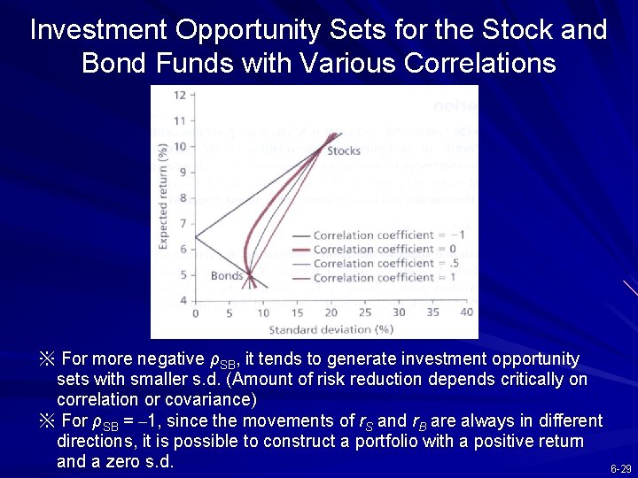
Investment Opportunity Sets for the Stock and Bond Funds with Various Correlations ※ For more negative ρSB, it tends to generate investment opportunity sets with smaller s. d. (Amount of risk reduction depends critically on correlation or covariance) ※ For ρSB = – 1, since the movements of r. S and r. B are always in different directions, it is possible to construct a portfolio with a positive return and a zero s. d. 6 -29

6. 3 THE OPTIMAL RISKY PORTFOLIO WITH A RISK-FREE ASSET 6 -30

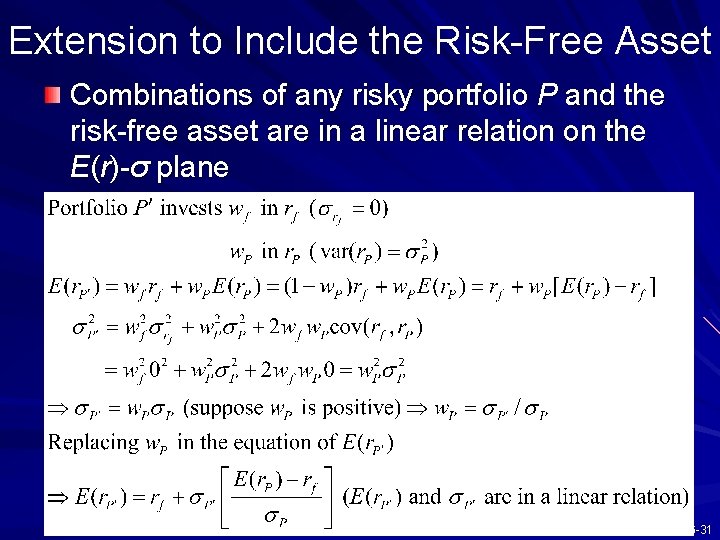
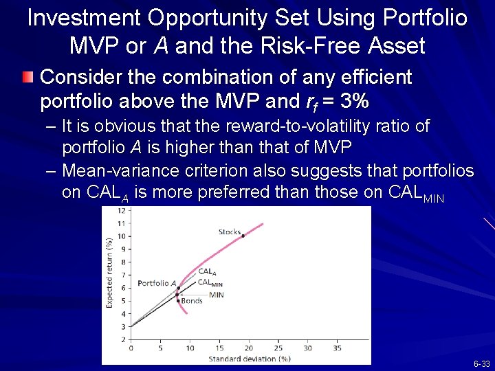
Extension to Include the Risk-Free Asset Combinations of any risky portfolio P and the risk-free asset are in a linear relation on the E(r)-σ plane 6 -31

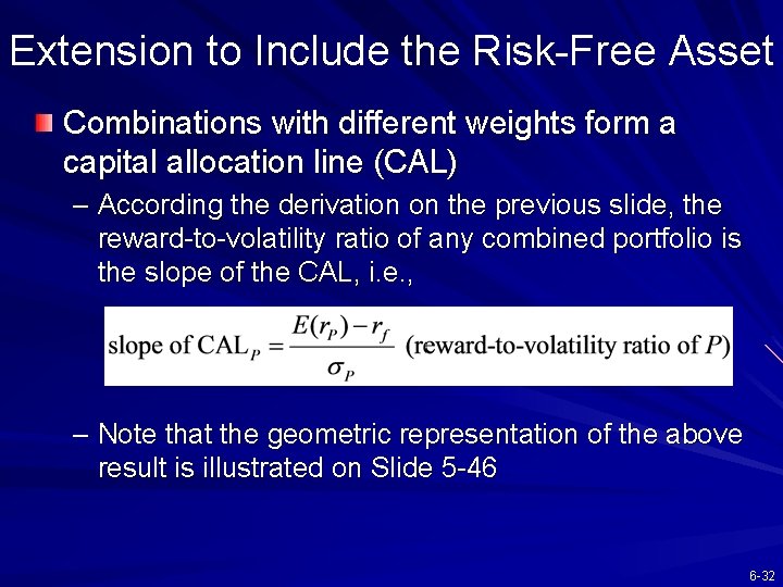
Extension to Include the Risk-Free Asset Combinations with different weights form a capital allocation line (CAL) – According the derivation on the previous slide, the reward-to-volatility ratio of any combined portfolio is the slope of the CAL, i. e. , – Note that the geometric representation of the above result is illustrated on Slide 5 -46 6 -32

Investment Opportunity Set Using Portfolio MVP or A and the Risk-Free Asset Consider the combination of any efficient portfolio above the MVP and rf = 3% – It is obvious that the reward-to-volatility ratio of portfolio A is higher than that of MVP – Mean-variance criterion also suggests that portfolios on CALA is more preferred than those on CALMIN 6 -33

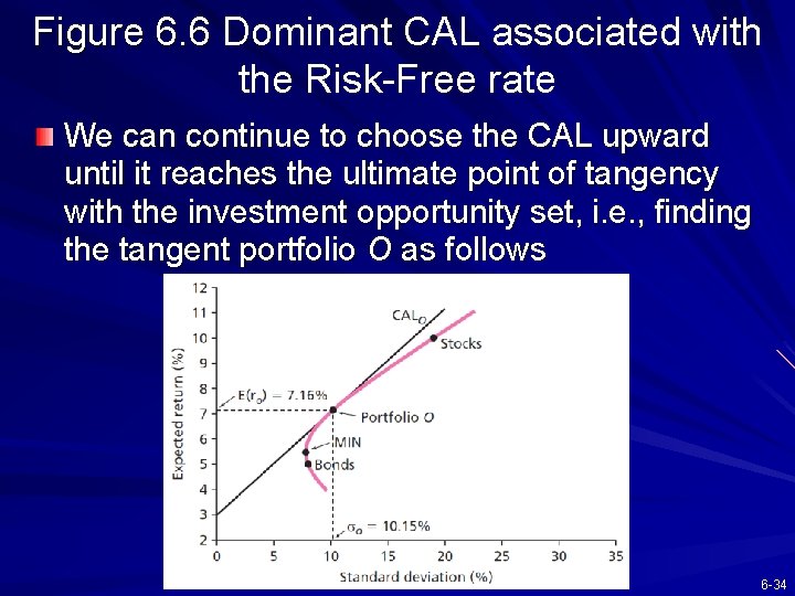
Figure 6. 6 Dominant CAL associated with the Risk-Free rate We can continue to choose the CAL upward until it reaches the ultimate point of tangency with the investment opportunity set, i. e. , finding the tangent portfolio O as follows 6 -34

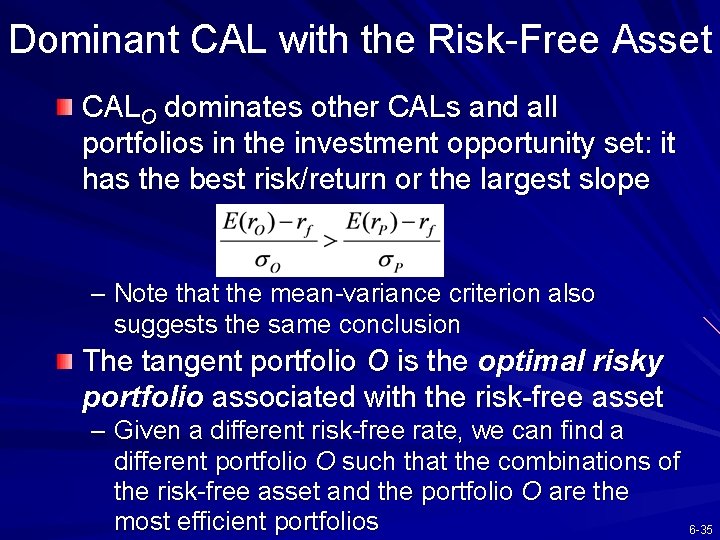
Dominant CAL with the Risk-Free Asset CALO dominates other CALs and all portfolios in the investment opportunity set: it has the best risk/return or the largest slope – Note that the mean-variance criterion also suggests the same conclusion The tangent portfolio O is the optimal risky portfolio associated with the risk-free asset – Given a different risk-free rate, we can find a different portfolio O such that the combinations of the risk-free asset and the portfolio O are the most efficient portfolios 6 -35

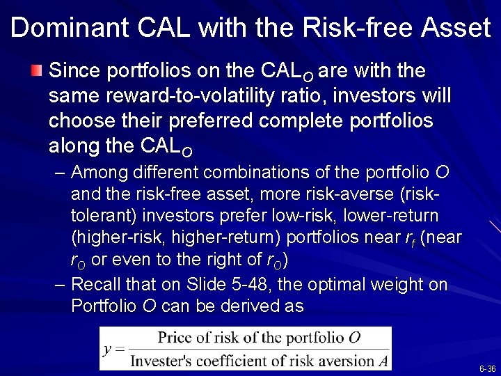
Dominant CAL with the Risk-free Asset Since portfolios on the CALO are with the same reward-to-volatility ratio, investors will choose their preferred complete portfolios along the CALO – Among different combinations of the portfolio O and the risk-free asset, more risk-averse (risktolerant) investors prefer low-risk, lower-return (higher-risk, higher-return) portfolios near rf (near r. O or even to the right of r. O) – Recall that on Slide 5 -48, the optimal weight on Portfolio O can be derived as 6 -36

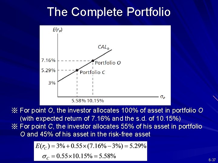
The Complete Portfolio ※ For point O, the investor allocates 100% of asset in portfolio O (with expected return of 7. 16% and the s. d. of 10. 15%) ※ For point C, the investor allocates 55% of his asset in portfolio O and 45% of his asset in the risk-free asset 6 -37

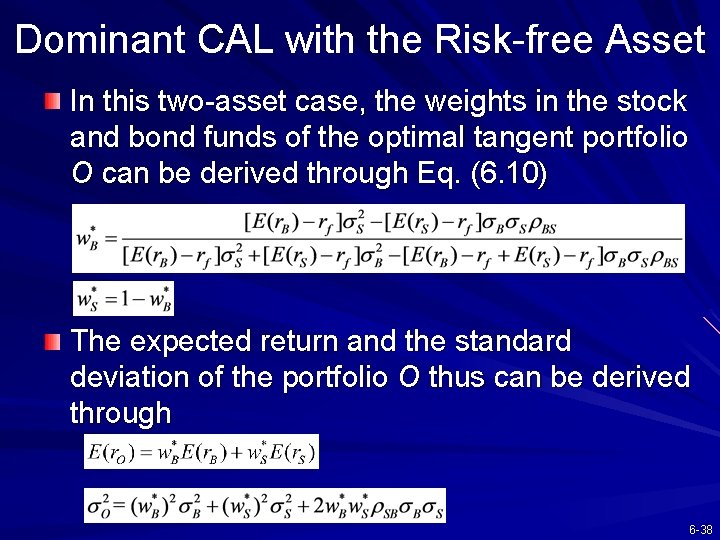
Dominant CAL with the Risk-free Asset In this two-asset case, the weights in the stock and bond funds of the optimal tangent portfolio O can be derived through Eq. (6. 10) The expected return and the standard deviation of the portfolio O thus can be derived through 6 -38

6. 4 EFFICIENT DIVERSIFICATION WITH MANY RISKY ASSETS 6 -39

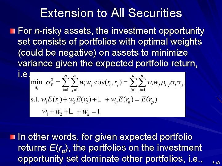
Extension to All Securities For n-risky assets, the investment opportunity set consists of portfolios with optimal weights (could be negative) on assets to minimize variance given the expected portfolio return, i. e. , In other words, for given expected portfolio returns E(rp), the portfolios on the investment opportunity set dominate other portfolios, i. e. , 6 -40

Extension to All Securities The curve for the investment opportunity set is also called the portfolio frontier (投資組合 前緣) The upper half of the portfolio frontier is called the efficient frontier (效率前緣), which represents a set of efficient portfolios that offer higher expected return at each level of portfolio risk (comparing to the lower half of the portfolio frontier) (see the next slide) 6 -41

The Efficient Frontier of Risky Assets and Individual Assets ※ For rational investors, they prefer the portfolio of risky assets on the efficient frontier due to the mean-variance criterion 6 -42

Extension to All Securities Using the current risk-free rate, we can search for the CAL with the highest reward-to-volatility ratio and thus find the optimal risky portfolio O (see Slides 6 -33 and 6 -34) Finally, investors choose the appropriate mix between the optimal risky portfolio O and the riskfree asset (see Slide 6 -37) The separation property: the process to choose portfolio combinations can be separated into two independent tasks 1. Determination of the optimal risky portfolio O, which is a purely technical problem 2. The personal choice of the mix of the risky portfolio and the risk-free asset depending on his preference 6 -43

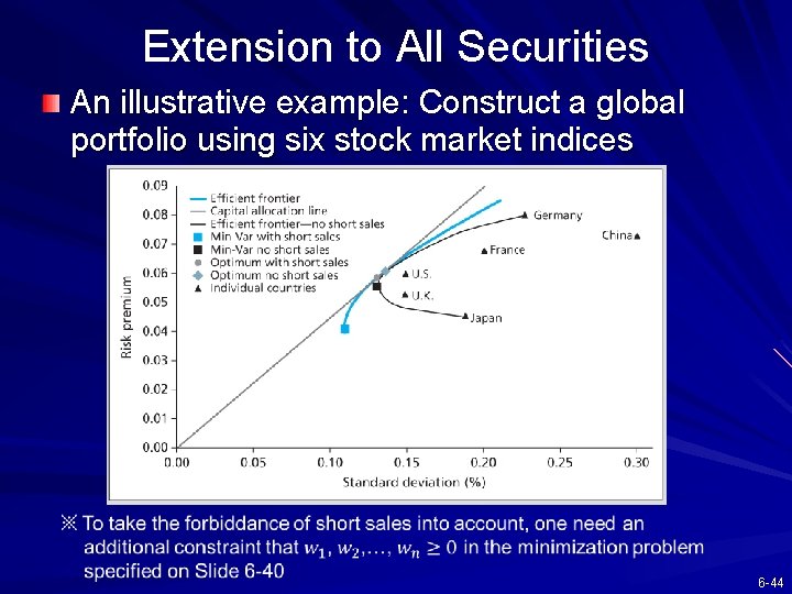
Extension to All Securities An illustrative example: Construct a global portfolio using six stock market indices 6 -44

6. 5 SINGLE-INDEX MODEL 6 -45

Index models The index model (指數模型) is a statistical model to measure or identify the components of firmspecific and systematic risks for a particular security or portfolio William Sharpe (1963), who is a Nobel Prize laureate in 1990, used the single-index model (單 一指數模型), also known as the market model (市 場模型), to explain the benefits of diversification – To separate the systematic and nonsystematic risks in the single-index model, it is intuitive to use the rate of return on a broad portfolio of securities, such as the S&P 500 index, as a proxy for the common macro factor (market risk factor) 6 -46

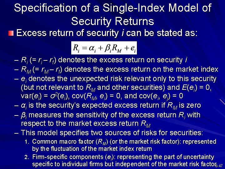
Specification of a Single-Index Model of Security Returns Excess return of security i can be stated as: – Ri (= ri – rf) denotes the excess return on security i – RM (= r. M – rf) denotes the excess return on the market index – ei denotes the unexpected risk relevant only to this security (but not relevant to RM and other securities) and E(ei) = 0, var(ei) = σ2(ei), cov(RM, ei) = 0, and cov(ei, ej) = 0 – αi is the security’s expected excess return if RM is zero – βi measures the sensitivity of the excess return Ri with respect to the market excess return RM – This model specifies two sources of risks for securities: 1. Common macro factor (RM) (or the market risk factor): represented by the fluctuation of the market index return 2. Firm-specific components (ei): representing the part of uncertainty specific to individual firms but independent of the market risk factor 6 -47

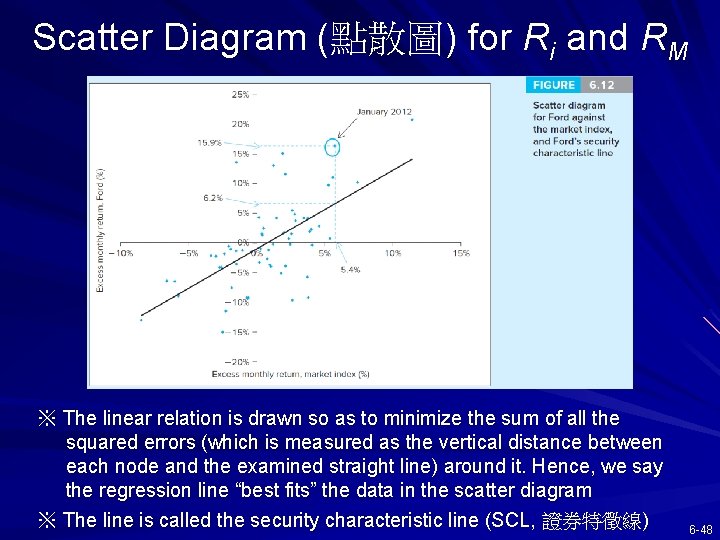
Scatter Diagram (點散圖) for Ri and RM ※ The linear relation is drawn so as to minimize the sum of all the squared errors (which is measured as the vertical distance between each node and the examined straight line) around it. Hence, we say the regression line “best fits” the data in the scatter diagram ※ The line is called the security characteristic line (SCL, 證券特徵線) 6 -48

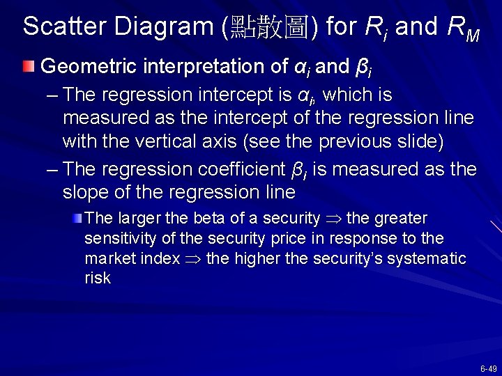
Scatter Diagram (點散圖) for Ri and RM Geometric interpretation of αi and βi – The regression intercept is αi, which is measured as the intercept of the regression line with the vertical axis (see the previous slide) – The regression coefficient βi is measured as the slope of the regression line The larger the beta of a security the greater sensitivity of the security price in response to the market index the higher the security’s systematic risk 6 -49

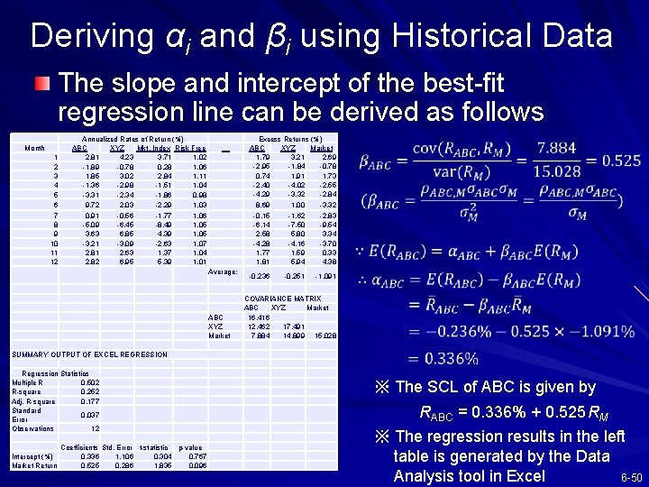
Deriving αi and βi using Historical Data The slope and intercept of the best-fit regression line can be derived as follows Month 1 2 3 4 5 6 7 8 9 10 11 12 Annualized Rates of Return (%) ABC XYZ Mkt. Index Risk Free 2. 81 4. 23 3. 71 1. 02 -1. 89 -0. 78 0. 28 1. 06 1. 85 3. 02 2. 84 1. 11 -1. 36 -2. 98 -1. 51 1. 04 -3. 31 -2. 34 -1. 86 0. 98 9. 72 2. 03 -2. 29 1. 03 0. 91 -0. 56 -1. 77 1. 06 -5. 09 -6. 45 -8. 49 1. 05 3. 63 6. 85 4. 39 1. 05 -3. 21 -3. 09 -2. 63 1. 07 2. 81 2. 63 1. 37 1. 04 2. 82 6. 95 5. 39 1. 01 Excess Returns (%) ABC XYZ Market 1. 79 3. 21 2. 69 -2. 95 -1. 84 -0. 78 0. 74 1. 91 1. 73 -2. 40 -4. 02 -2. 55 -4. 29 -3. 32 -2. 84 8. 69 1. 00 -3. 32 -0. 15 -1. 62 -2. 83 -6. 14 -7. 50 -9. 54 2. 58 5. 80 3. 34 -4. 28 -4. 16 -3. 70 1. 77 1. 59 0. 33 1. 81 5. 94 4. 38 Average: ABC XYZ Market -0. 236 -0. 251 -1. 091 COVARIANCE MATRIX ABC XYZ Market 16. 416 12. 462 17. 491 7. 884 14. 899 15. 028 SUMMARY OUTPUT OF EXCEL REGRESSION Regression Statistics Multiple R 0. 502 R-square 0. 252 Adj. R-square 0. 177 Standard 0. 037 Error Observations 12 Coefficients Std. Error t-statistic p-value Intercept (%) 0. 336 1. 106 0. 304 0. 767 Market Return 0. 525 0. 286 1. 835 0. 096 ※ The SCL of ABC is given by RABC = 0. 336% + 0. 525 RM ※ The regression results in the left table is generated by the Data Analysis tool in Excel 6 -50

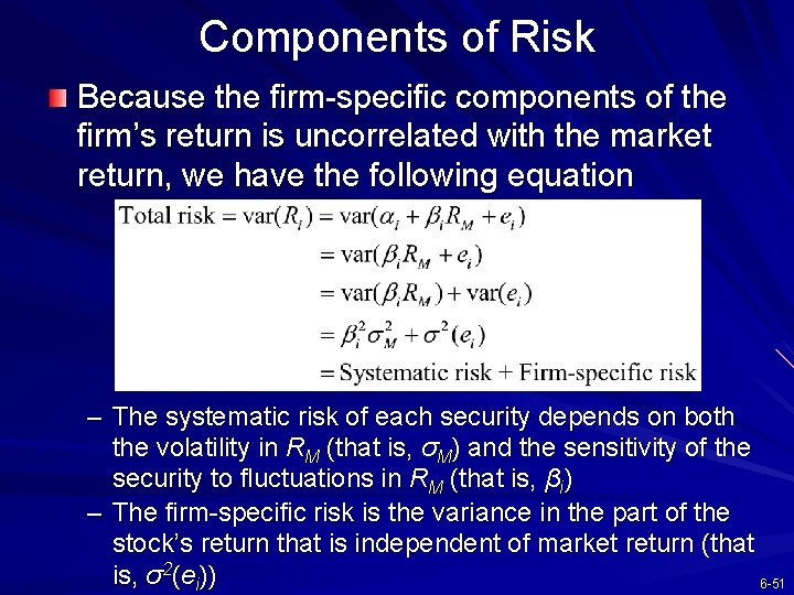
Components of Risk Because the firm-specific components of the firm’s return is uncorrelated with the market return, we have the following equation – The systematic risk of each security depends on both the volatility in RM (that is, σM) and the sensitivity of the security to fluctuations in RM (that is, βi) – The firm-specific risk is the variance in the part of the stock’s return that is independent of market return (that is, σ2(ei)) 6 -51

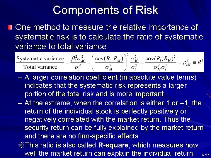
Components of Risk One method to measure the relative importance of systematic risk is to calculate the ratio of systematic variance to total variance – A larger correlation coefficient (in absolute value terms) indicates that the systematic risk represents a larger portion of the total risk and is more important – At the extreme, when the correlation is either 1 or – 1, the return of the individual stock is perfectly positively or negatively correlated with the market return. Thus the security return can be fully explained by the market return and there are no firm-specific effects ※This ratio is also called R-square, which measures how well the market return can explain the individual return 6 -52

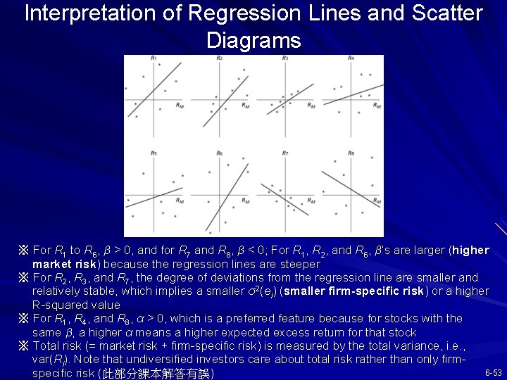
Interpretation of Regression Lines and Scatter Diagrams ※ For R 1 to R 6, β > 0, and for R 7 and R 8, β < 0; For R 1, R 2, and R 6, β’s are larger (higher market risk) because the regression lines are steeper ※ For R 2, R 3, and R 7, the degree of deviations from the regression line are smaller and relatively stable, which implies a smaller σ2(ei) (smaller firm-specific risk) or a higher R-squared value ※ For R 1, R 4, and R 8, α > 0, which is a preferred feature because for stocks with the same β, a higher α means a higher expected excess return for that stock ※ Total risk (= market risk + firm-specific risk) is measured by the total variance, i. e. , var(Ri). Note that undiversified investors care about total risk rather than only firm 6 -53 specific risk (此部分課本解答有誤)

Predicting Betas The beta from the regression equation is an estimate based on past history, but we want to forecast beta in the future Betas exhibit a statistical property called “regression toward the mean” (向平均回歸) – High (low) beta (that is beta > (<) 1) securities in one period tend to exhibit a lower (higher) beta in the future (Blume (1975)) Adjusted betas (proposed by Klemkosky and Martin (1975) and adopted by Merrill Lynch) – A common weighting scheme is 2/3 on the historical estimate and 1/3 on the value of 1 – Based on the results of ABC on Slide 6 -50, the adjusted beta is (2/3)× 0. 525+(1/3)× 1=0. 6833 6 -54

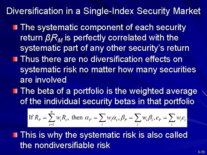
Diversification in a Single-Index Security Market The systematic component of each security return βi. RM is perfectly correlated with the systematic part of any other security’s return Thus there are no diversification effects on systematic risk no matter how many securities are involved The beta of a portfolio is the weighted average of the individual security betas in that portfolio This is why the systematic risk is also called the nondiversifiable risk 6 -55

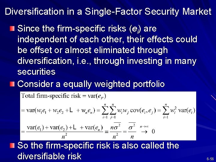
Diversification in a Single-Factor Security Market Since the firm-specific risks (ei) are independent of each other, their effects could be offset or almost eliminated through diversification, i. e. , through investing in many securities Consider a equally weighted portfolio So the firm-specific risk is also called the diversifiable risk 6 -56

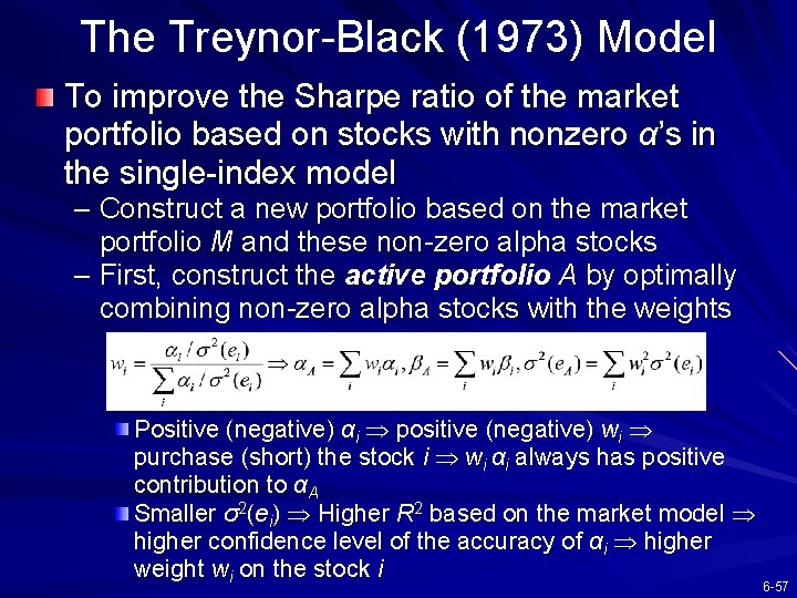
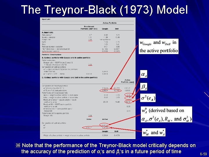
The Treynor-Black (1973) Model To improve the Sharpe ratio of the market portfolio based on stocks with nonzero α’s in the single-index model – Construct a new portfolio based on the market portfolio M and these non-zero alpha stocks – First, construct the active portfolio A by optimally combining non-zero alpha stocks with the weights Positive (negative) αi positive (negative) wi purchase (short) the stock i wi αi always has positive contribution to αA Smaller σ2(ei) Higher R 2 based on the market model higher confidence level of the accuracy of αi higher weight wi on the stock i 6 -57

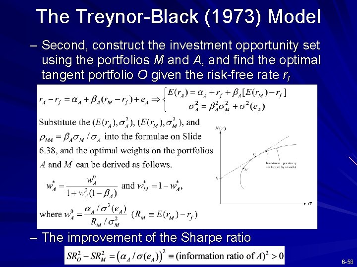
The Treynor-Black (1973) Model – Second, construct the investment opportunity set using the portfolios M and A, and find the optimal tangent portfolio O given the risk-free rate rf – The improvement of the Sharpe ratio 6 -58

The Treynor-Black (1973) Model ※ Note that the performance of the Treynor-Black model critically depends on the accuracy of the prediction of αi‘s and βi‘s in a future period of time 6 -59

6. 6 RISK OF LONG-TERM INVESTMENTS 6 -60

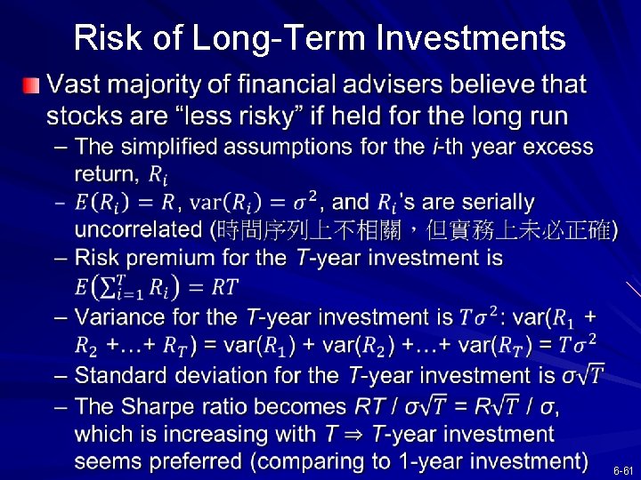
Risk of Long-Term Investments 6 -61

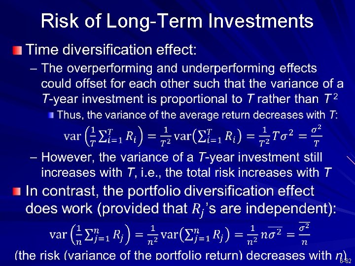
Risk of Long-Term Investments 6 -62