CHAPTER 6 Efficient Diversification Mc GrawHillIrwin Copyright 2008

CHAPTER 6 Efficient Diversification Mc. Graw-Hill/Irwin Copyright © 2008 The Mc. Graw-Hill Companies, Inc. , All Rights Reserved.

6. 1 DIVERSIFICATION AND PORTFOLIO RISK 6 -2

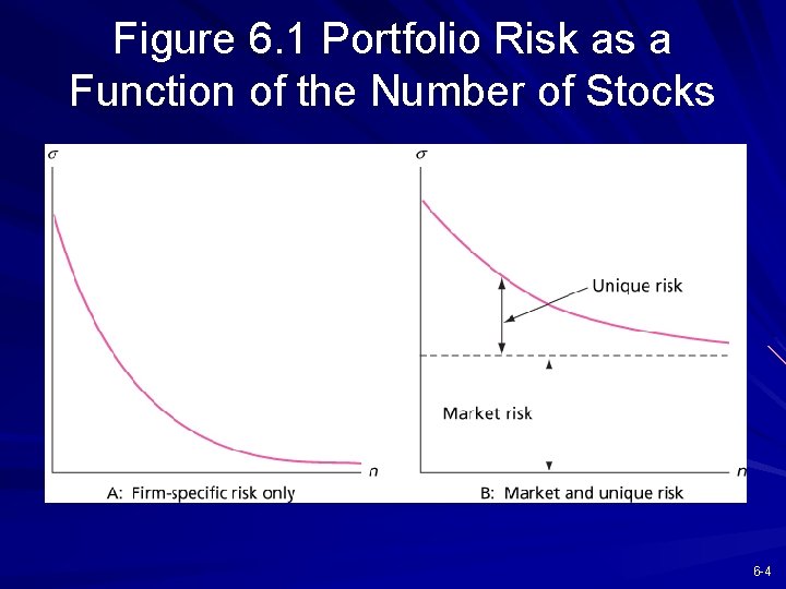
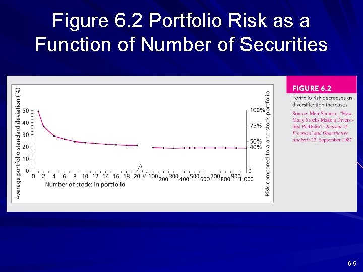
Diversification and Portfolio Risk Market risk – Systematic or Nondiversifiable Firm-specific risk – Diversifiable or nonsystematic 6 -3

Figure 6. 1 Portfolio Risk as a Function of the Number of Stocks 6 -4

Figure 6. 2 Portfolio Risk as a Function of Number of Securities 6 -5

6. 2 ASSET ALLOCATION WITH TWO RISKY ASSETS 6 -6

Covariance and Correlation Portfolio risk depends on the correlation between the returns of the assets in the portfolio Covariance and the correlation coefficient provide a measure of the returns on two assets to vary 6 -7

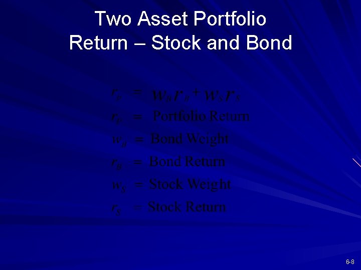
Two Asset Portfolio Return – Stock and Bond 6 -8

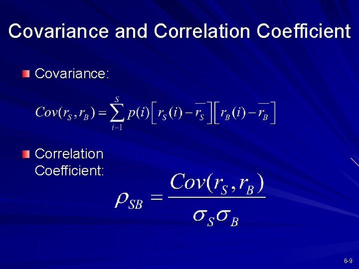
Covariance and Correlation Coefficient Covariance: Correlation Coefficient: 6 -9

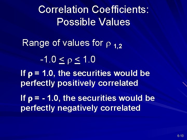
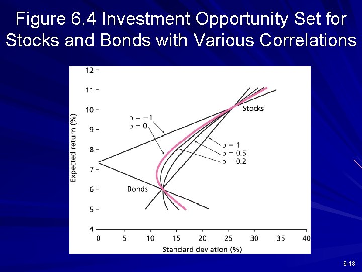
Correlation Coefficients: Possible Values Range of values for r 1, 2 -1. 0 < r < 1. 0 If r = 1. 0, the securities would be perfectly positively correlated If r = - 1. 0, the securities would be perfectly negatively correlated 6 -10

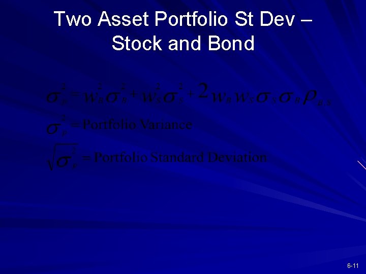
Two Asset Portfolio St Dev – Stock and Bond 6 -11

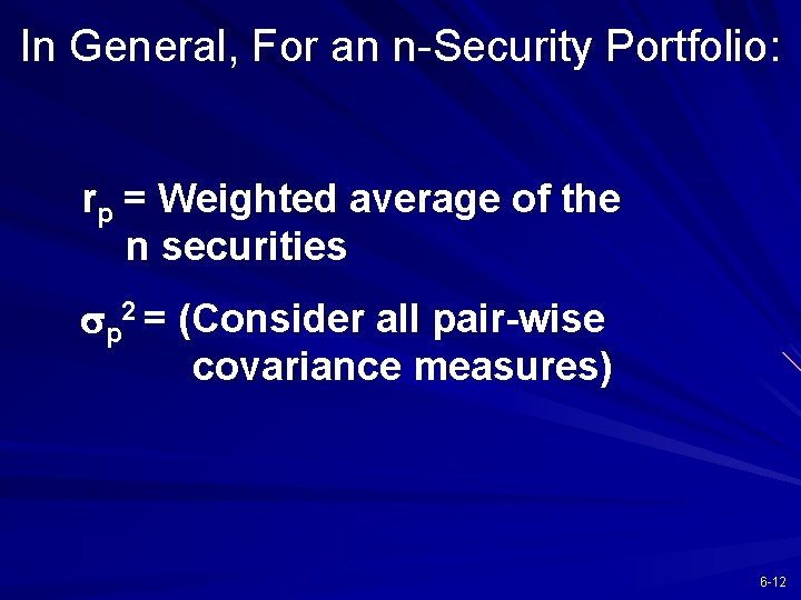
In General, For an n-Security Portfolio: rp = Weighted average of the n securities sp 2 = (Consider all pair-wise covariance measures) 6 -12

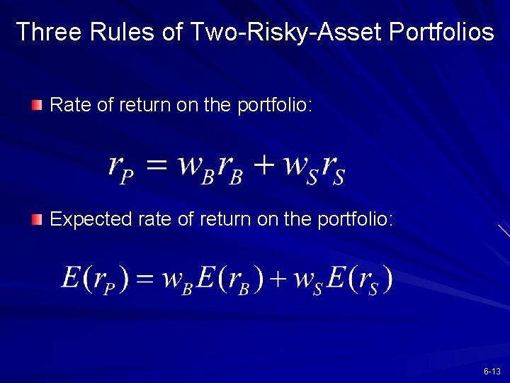
Three Rules of Two-Risky-Asset Portfolios Rate of return on the portfolio: Expected rate of return on the portfolio: 6 -13

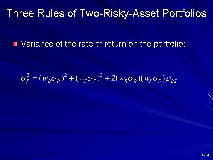
Three Rules of Two-Risky-Asset Portfolios Variance of the rate of return on the portfolio: 6 -14

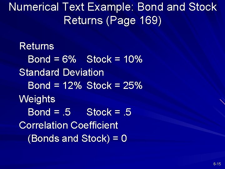
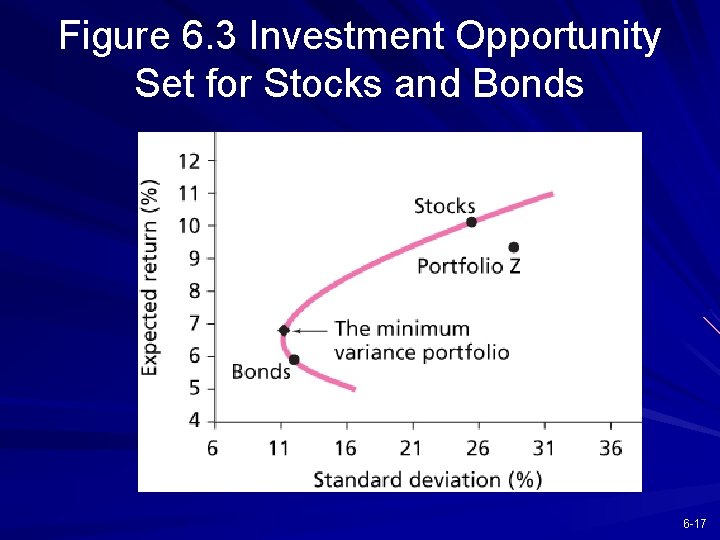
Numerical Text Example: Bond and Stock Returns (Page 169) Returns Bond = 6% Stock = 10% Standard Deviation Bond = 12% Stock = 25% Weights Bond =. 5 Stock =. 5 Correlation Coefficient (Bonds and Stock) = 0 6 -15

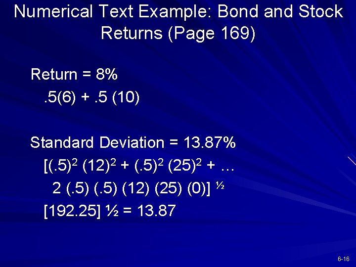
Numerical Text Example: Bond and Stock Returns (Page 169) Return = 8%. 5(6) +. 5 (10) Standard Deviation = 13. 87% [(. 5)2 (12)2 + (. 5)2 (25)2 + … 2 (. 5) (12) (25) (0)] ½ [192. 25] ½ = 13. 87 6 -16

Figure 6. 3 Investment Opportunity Set for Stocks and Bonds 6 -17

Figure 6. 4 Investment Opportunity Set for Stocks and Bonds with Various Correlations 6 -18

6. 3 THE OPTIMAL RISKY PORTFOLIO WITH A RISK-FREE ASSET 6 -19

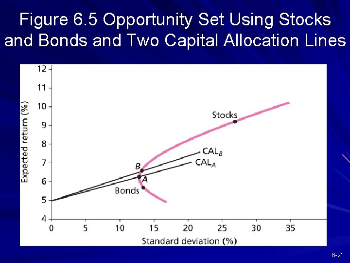
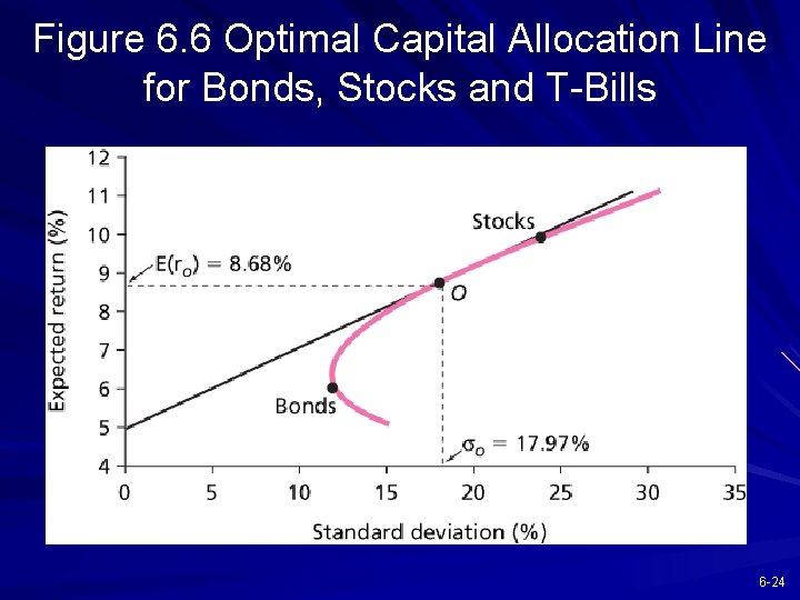
Extending to Include Riskless Asset The optimal combination becomes linear A single combination of risky and riskless assets will dominate 6 -20

Figure 6. 5 Opportunity Set Using Stocks and Bonds and Two Capital Allocation Lines 6 -21

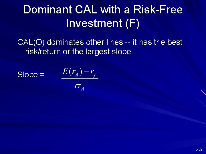
Dominant CAL with a Risk-Free Investment (F) CAL(O) dominates other lines -- it has the best risk/return or the largest slope Slope = 6 -22

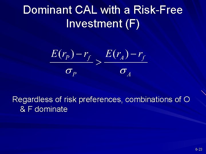
Dominant CAL with a Risk-Free Investment (F) Regardless of risk preferences, combinations of O & F dominate 6 -23

Figure 6. 6 Optimal Capital Allocation Line for Bonds, Stocks and T-Bills 6 -24

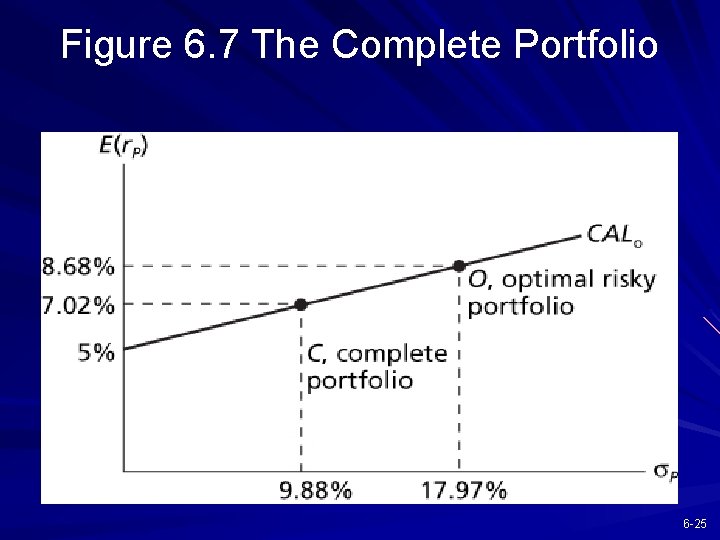
Figure 6. 7 The Complete Portfolio 6 -25

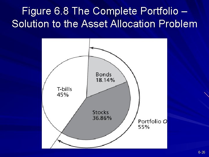
Figure 6. 8 The Complete Portfolio – Solution to the Asset Allocation Problem 6 -26

6. 4 EFFICIENT DIVERSIFICATION WITH MANY RISKY ASSETS 6 -27

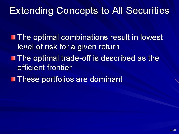
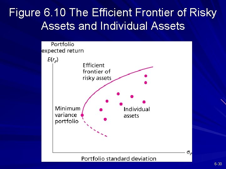
Extending Concepts to All Securities The optimal combinations result in lowest level of risk for a given return The optimal trade-off is described as the efficient frontier These portfolios are dominant 6 -28

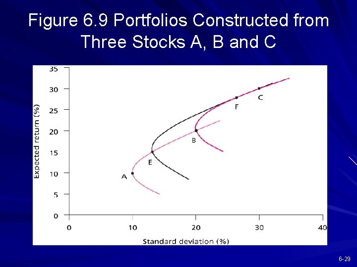
Figure 6. 9 Portfolios Constructed from Three Stocks A, B and C 6 -29

Figure 6. 10 The Efficient Frontier of Risky Assets and Individual Assets 6 -30

6. 5 A SINGLE-FACTOR ASSET MARKET 6 -31

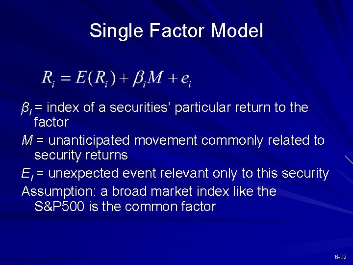
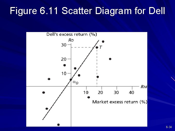
Single Factor Model βi = index of a securities’ particular return to the factor M = unanticipated movement commonly related to security returns Ei = unexpected event relevant only to this security Assumption: a broad market index like the S&P 500 is the common factor 6 -32

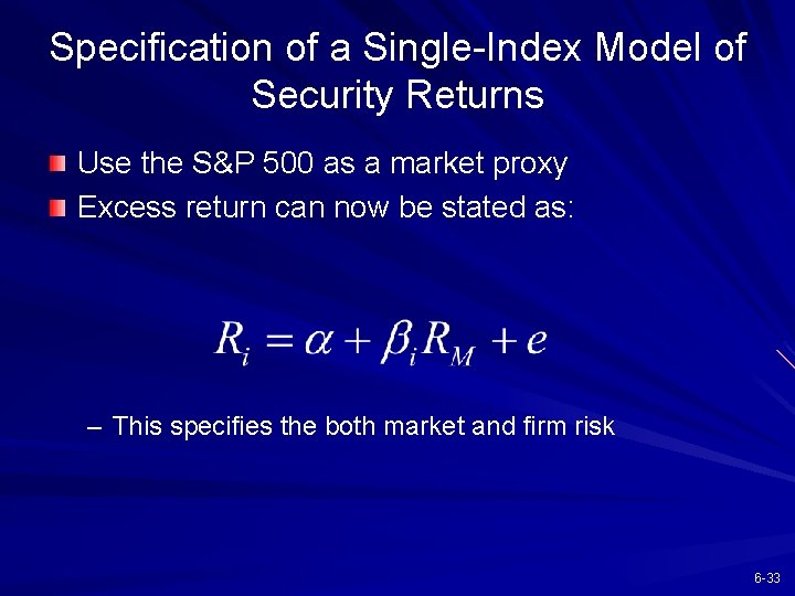
Specification of a Single-Index Model of Security Returns Use the S&P 500 as a market proxy Excess return can now be stated as: – This specifies the both market and firm risk 6 -33

Figure 6. 11 Scatter Diagram for Dell 6 -34

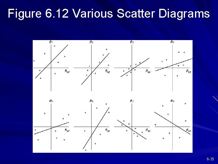
Figure 6. 12 Various Scatter Diagrams 6 -35

Components of Risk Market or systematic risk: risk related to the macro economic factor or market index Unsystematic or firm specific risk: risk not related to the macro factor or market index Total risk = Systematic + Unsystematic 6 -36

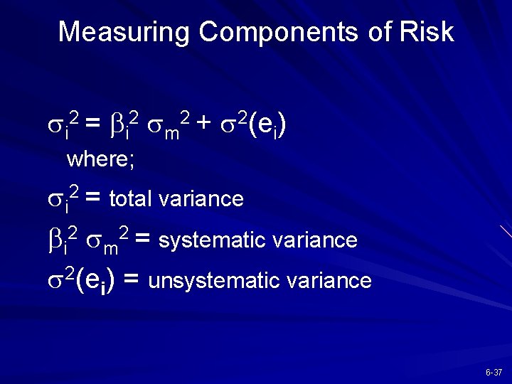
Measuring Components of Risk si 2 = bi 2 sm 2 + s 2(ei) where; si 2 = total variance bi 2 sm 2 = systematic variance s 2(ei) = unsystematic variance 6 -37

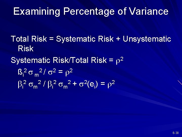
Examining Percentage of Variance Total Risk = Systematic Risk + Unsystematic Risk Systematic Risk/Total Risk = r 2 ß i 2 s m 2 / s 2 = r 2 bi 2 sm 2 / bi 2 sm 2 + s 2(ei) = r 2 6 -38

Advantages of the Single Index Model Reduces the number of inputs for diversification Easier for security analysts to specialize 6 -39

6. 6 RISK OF LONG-TERM INVESTMENTS 6 -40

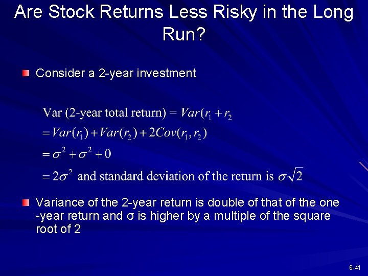
Are Stock Returns Less Risky in the Long Run? Consider a 2 -year investment Variance of the 2 -year return is double of that of the one -year return and σ is higher by a multiple of the square root of 2 6 -41

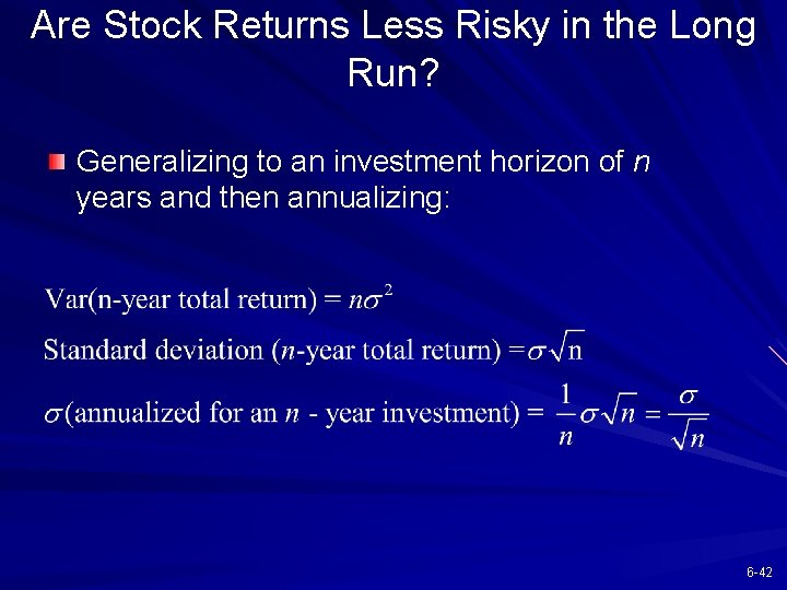
Are Stock Returns Less Risky in the Long Run? Generalizing to an investment horizon of n years and then annualizing: 6 -42

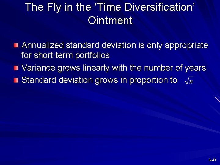
The Fly in the ‘Time Diversification’ Ointment Annualized standard deviation is only appropriate for short-term portfolios Variance grows linearly with the number of years Standard deviation grows in proportion to 6 -43

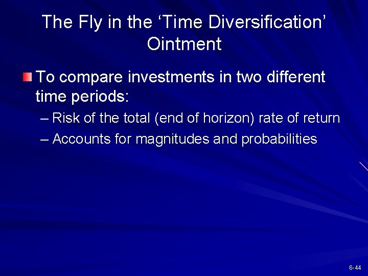
The Fly in the ‘Time Diversification’ Ointment To compare investments in two different time periods: – Risk of the total (end of horizon) rate of return – Accounts for magnitudes and probabilities 6 -44