Chapter 6 Efficient Diversification Mc GrawHillIrwin Copyright 2010

Chapter 6 Efficient Diversification Mc. Graw-Hill/Irwin Copyright © 2010 by The Mc. Graw-Hill Companies, Inc. All rights reserved.

Chapter 6 Efficient Diversification 6 -2

6. 1 Diversification and Portfolio Risk 6. 2 Asset Allocation With Two Risky Assets 6 -3

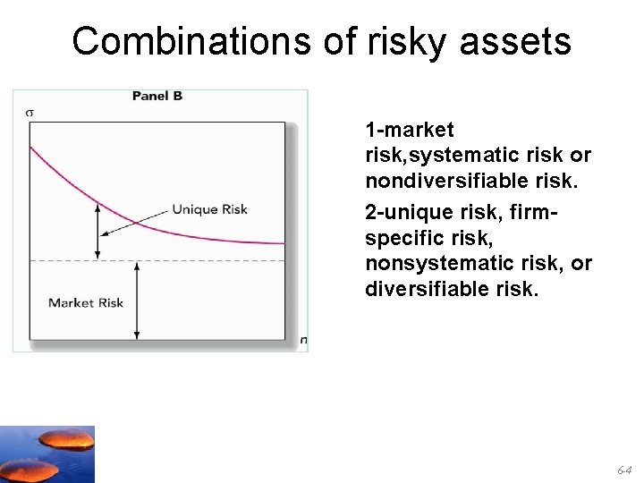
Combinations of risky assets 1 -market risk, systematic risk or nondiversifiable risk. 2 -unique risk, firmspecific risk, nonsystematic risk, or diversifiable risk. 6 -4

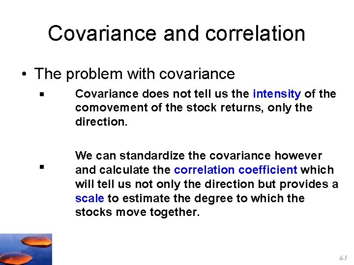
Covariance and correlation • The problem with covariance § § Covariance does not tell us the intensity of the comovement of the stock returns, only the direction. We can standardize the covariance however and calculate the correlation coefficient which will tell us not only the direction but provides a scale to estimate the degree to which the stocks move together. 6 -5

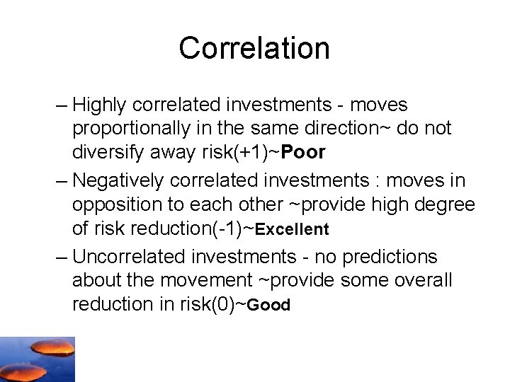
Correlation – Highly correlated investments - moves proportionally in the same direction~ do not diversify away risk(+1)~Poor – Negatively correlated investments : moves in opposition to each other ~provide high degree of risk reduction(-1)~Excellent – Uncorrelated investments - no predictions about the movement ~provide some overall reduction in risk(0)~Good

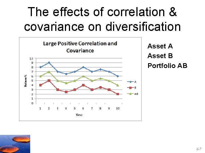
The effects of correlation & covariance on diversification Asset A Asset B Portfolio AB 6 -7

The effects of correlation & covariance on diversification Asset C Portfolio CD 6 -8

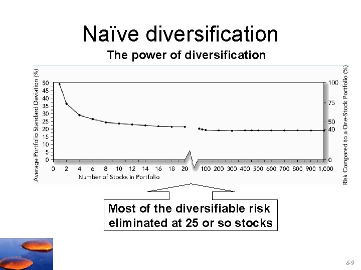
Naïve diversification The power of diversification Most of the diversifiable risk eliminated at 25 or so stocks 6 -9

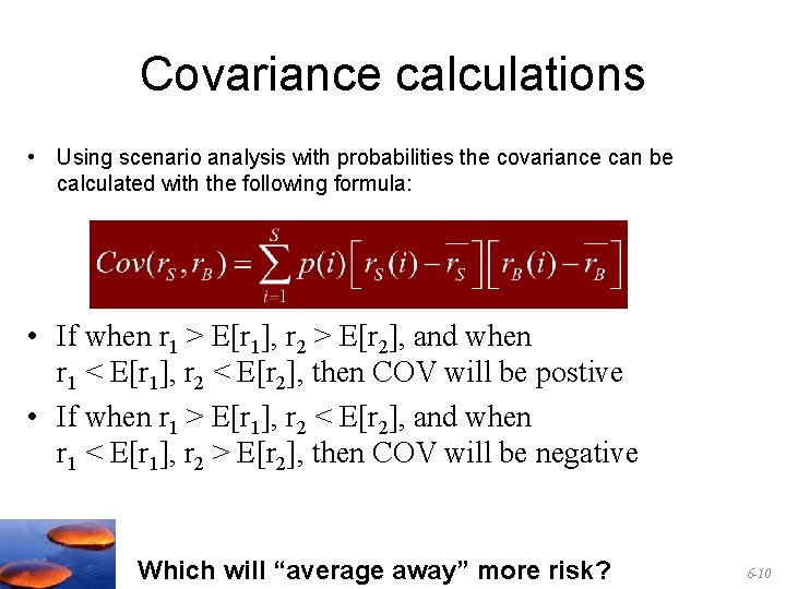
Covariance calculations • Using scenario analysis with probabilities the covariance can be calculated with the following formula: • If when r 1 > E[r 1], r 2 > E[r 2], and when r 1 < E[r 1], r 2 < E[r 2], then COV will be postive • If when r 1 > E[r 1], r 2 < E[r 2], and when r 1 < E[r 1], r 2 > E[r 2], then COV will be negative Which will “average away” more risk? 6 -10

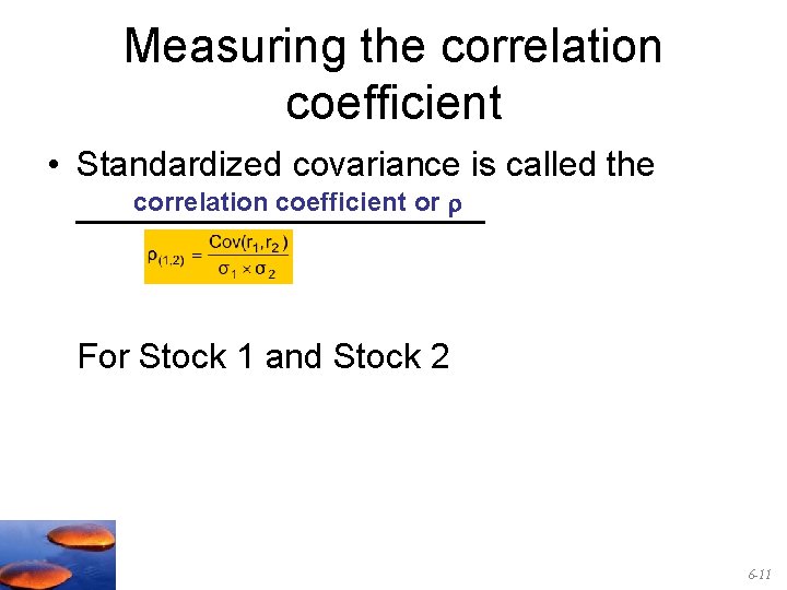
Measuring the correlation coefficient • Standardized covariance is called the correlation coefficient or ___________ For Stock 1 and Stock 2 6 -11

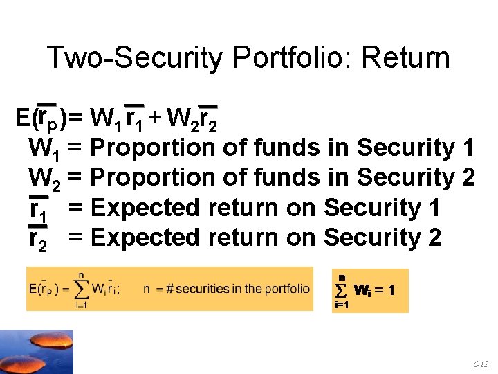
Two-Security Portfolio: Return rp = W 1 r 1 + W 2 r 2 E( ) W 1 = Proportion of funds in Security 1 W 2 = Proportion of funds in Security 2 r 1 = Expected return on Security 1 r 2 = Expected return on Security 2 6 -12

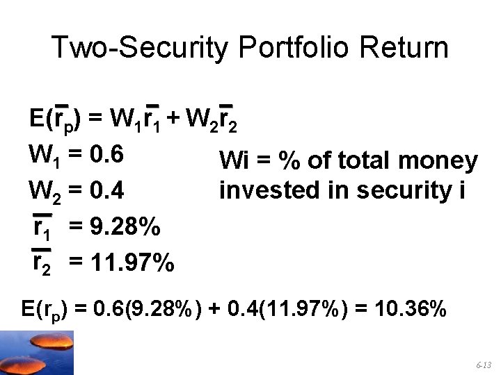
Two-Security Portfolio Return E(rp) = W 1 r 1 + W 2 r 2 W 1 = 0. 6 Wi = % of total money W 2 = 0. 4 invested in security i r 1 = 9. 28% r 2 = 11. 97% E(rp) = 0. 6(9. 28%) + 0. 4(11. 97%) = 10. 36% 6 -13

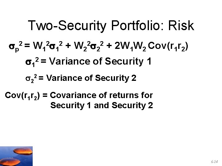
Two-Security Portfolio: Risk p 2 = W 12 12 + W 22 22 + 2 W 1 W 2 Cov(r 1 r 2) 12 = Variance of Security 1 22 = Variance of Security 2 Cov(r 1 r 2) = Covariance of returns for Security 1 and Security 2 6 -14

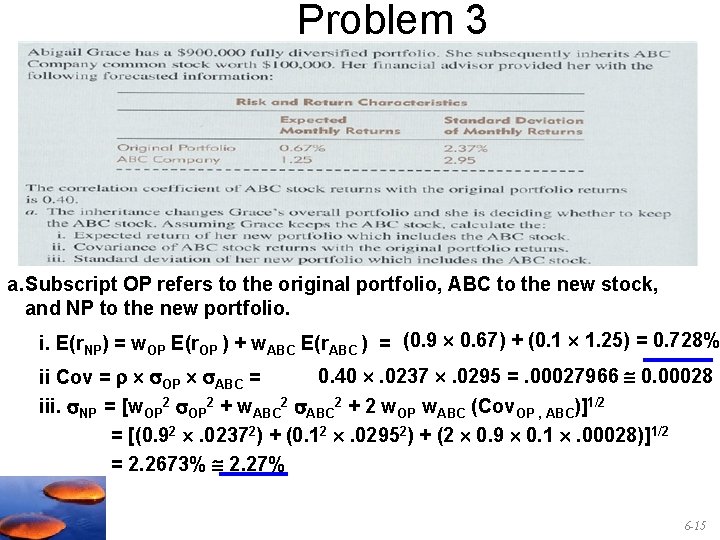
Problem 3 a. Subscript OP refers to the original portfolio, ABC to the new stock, and NP to the new portfolio. i. E(r. NP) = w. OP E(r. OP ) + w. ABC E(r. ABC ) = (0. 9 0. 67) + (0. 1 1. 25) = 0. 728% 0. 40 . 0237 . 0295 =. 00027966 0. 00028 ii Cov = OP ABC = iii. NP = [w. OP 2 + w. ABC 2 + 2 w. OP w. ABC (Cov. OP , ABC)]1/2 = [(0. 92 . 02372) + (0. 12 . 02952) + (2 0. 9 0. 1 . 00028)]1/2 = 2. 2673% 2. 27% 6 -15

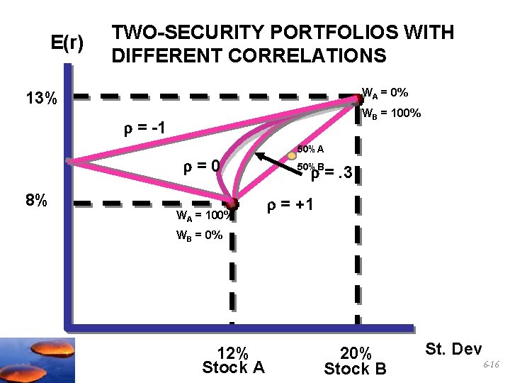
E(r) TWO-SECURITY PORTFOLIOS WITH DIFFERENT CORRELATIONS WA = 0% 13% WB = 100% = -1 = 0 8% WA = 100% 50%A =. 3 50%B = +1 WB = 0% 12% Stock A 20% Stock B St. Dev 6 -16

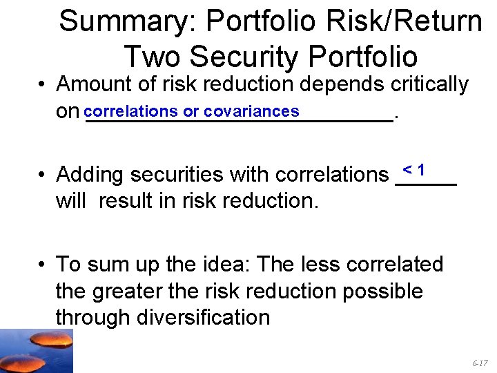
Summary: Portfolio Risk/Return Two Security Portfolio • Amount of risk reduction depends critically on correlations or covariances _____________. < 1 • Adding securities with correlations _____ will result in risk reduction. • To sum up the idea: The less correlated the greater the risk reduction possible through diversification 6 -17

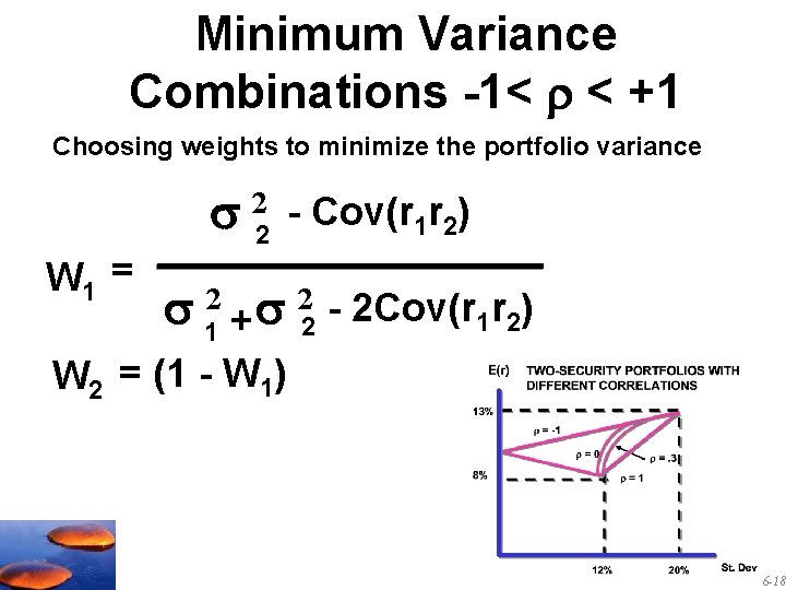
Minimum Variance Combinations -1< < +1 Choosing weights to minimize the portfolio variance W 1 = 2 - Cov(r 2 1 r 2) 12 + 22 - 2 Cov(r 1 r 2) W 2 = (1 - W 1) 6 -18

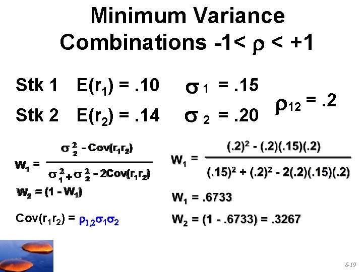
Minimum Variance Combinations -1< < +1 Stk 1 E(r 1) =. 10 Stk 2 E(r 2) =. 14 1 =. 15 12 =. 2 2 =. 20 Cov(r 1 r 2) = 1, 2 1 2 6 -19

Minimum Variance: Return and Risk with r =. 2 1 E[rp] =. 6733(. 10) +. 3267(. 14) =. 1131 or 11. 31% p 2 = W 12 12 + W 22 22 + 2 W 1 W 2 1, 2 1 2 6 -20

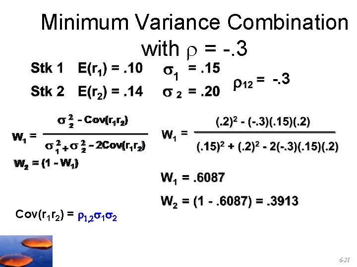
Minimum Variance Combination with r = -. 3 1 -. 3 Cov(r 1 r 2) = 1, 2 1 2 6 -21

Minimum Variance Combination with r = -. 3 1 -. 3 E[rp] = 0. 6087(. 10) + 0. 3913(. 14) =. 1157 = 11. 57% p 2 = W 12 12 + W 22 22 + 2 W 1 W 2 1, 2 1 2 Notice lower portfolio standard deviation but higher expected return with smaller 12 =. 2 E(rp) = 11. 31% p = 13. 08% 6 -22

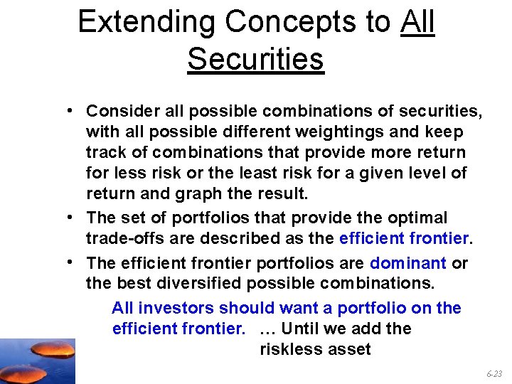
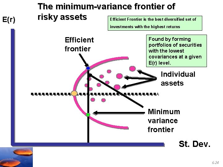
Extending Concepts to All Securities • Consider all possible combinations of securities, with all possible different weightings and keep track of combinations that provide more return for less risk or the least risk for a given level of return and graph the result. • The set of portfolios that provide the optimal trade-offs are described as the efficient frontier. • The efficient frontier portfolios are dominant or the best diversified possible combinations. All investors should want a portfolio on the efficient frontier. … Until we add the riskless asset 6 -23

E(r) The minimum-variance frontier of risky assets Efficient Frontier is the best diversified set of investments with the highest returns Efficient frontier Found by forming portfolios of securities with the lowest covariances at a given E(r) level. Individual assets Minimum variance frontier St. Dev. 6 -24

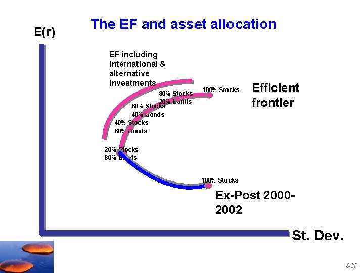
E(r) The EF and asset allocation EF including international & alternative investments 80% Stocks 20% Bonds 60% Stocks 40% Bonds 40% Stocks 60% Bonds 100% Stocks Efficient frontier 20% Stocks 80% Bonds 100% Stocks Ex-Post 20002002 St. Dev. 6 -25

6. 3 The Optimal Risky Portfolio With A Risk-Free Asset 6. 4 Efficient Diversification With Many Risky Assets 6 -26

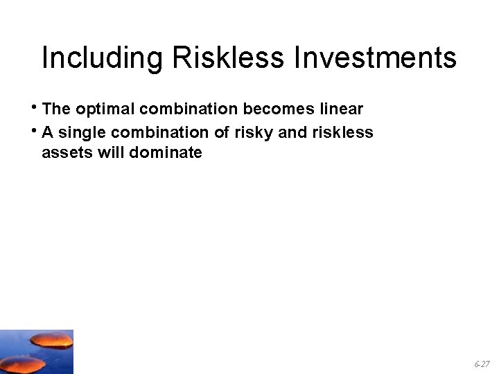
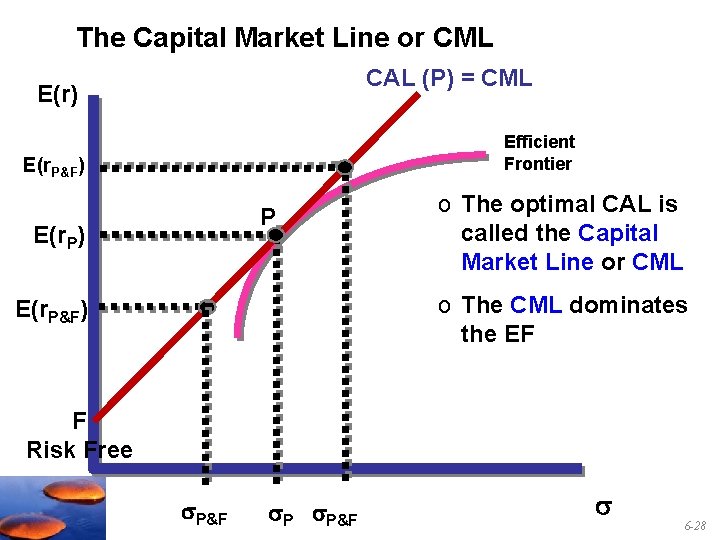
Including Riskless Investments • The optimal combination becomes linear • A single combination of risky and riskless assets will dominate 6 -27

The Capital Market Line or CML CAL (P) = CML E(r) Efficient Frontier E(r. P&F) P E(r. P) o The optimal CAL is called the Capital Market Line or CML o The CML dominates the EF E(r. P&F) F Risk Free P&F P P&F 6 -28

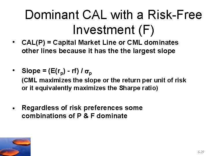
Dominant CAL with a Risk-Free Investment (F) • CAL(P) = Capital Market Line or CML dominates other lines because it has the largest slope • Slope = (E(rp) - rf) / p (CML maximizes the slope or the return per unit of risk or it equivalently maximizes the Sharpe ratio) • Regardless of risk preferences some combinations of P & F dominate 6 -29

6. 5 A Single Index Asset Market 6 -30

Individual securities We have learned that investors should diversify. Individual securities will be held in a portfolio. Consequently, the relevant risk of an individual security is the risk that remains when the security is placed in a portfolio. What do we call the risk that cannot be diversified away, i. e. , the risk that remains when the stock is put into a portfolio? Systematic risk How do we measure a stock’s systematic risk? 6 -31

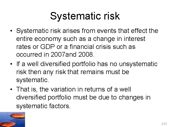
Systematic risk • Systematic risk arises from events that effect the entire economy such as a change in interest rates or GDP or a financial crisis such as occurred in 2007 and 2008. • If a well diversified portfolio has no unsystematic risk then any risk that remains must be systematic. • That is, the variation in returns of a well diversified portfolio must be due to changes in systematic factors. 6 -32

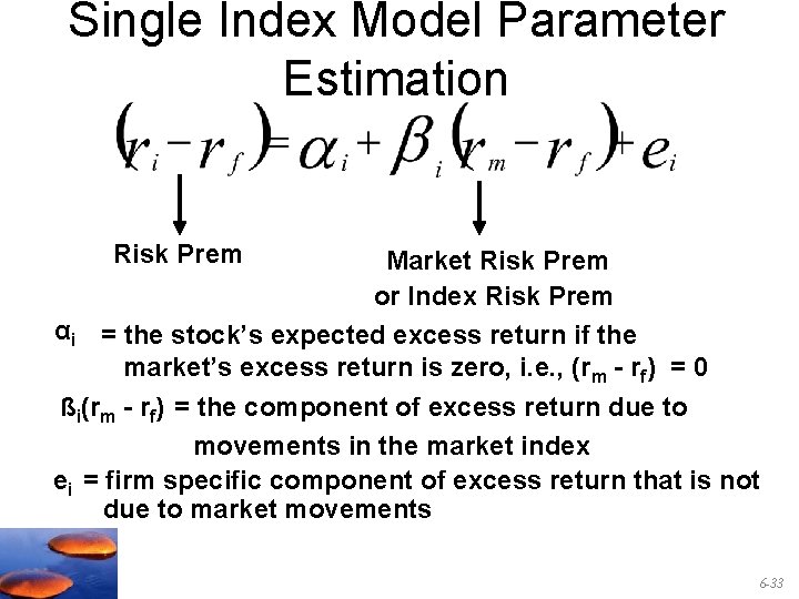
Single Index Model Parameter Estimation Risk Prem Market Risk Prem or Index Risk Prem αi = the stock’s expected excess return if the market’s excess return is zero, i. e. , (rm - rf) = 0 ßi(rm - rf) = the component of excess return due to movements in the market index ei = firm specific component of excess return that is not due to market movements 6 -33

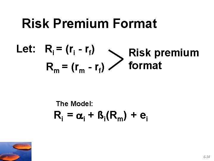
Risk Premium Format Let: Ri = (ri - rf) Rm = (rm - rf) Risk premium format The Model: Ri = ai + ßi(Rm) + ei 6 -34

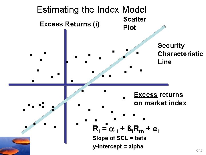
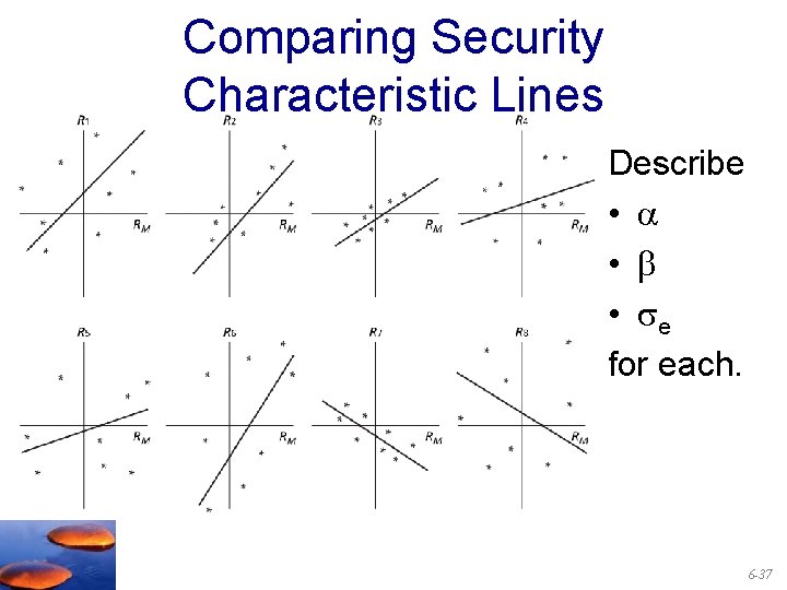
Estimating the Index Model Scatter Plot Excess Returns (i) . . Security. . Characteristic. . . Line. . Excess returns. . on market index. . . . R = a . + ß R + e i i i m Slope of SCL = beta y-intercept = alpha i 6 -35

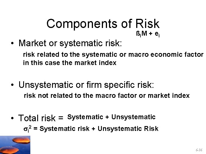
Components of Risk • Market or systematic risk: ßi. M + ei risk related to the systematic or macro economic factor in this case the market index • Unsystematic or firm specific risk: risk not related to the macro factor or market index • Total risk = Systematic + Unsystematic i 2 = Systematic risk + Unsystematic Risk 6 -36

Comparing Security Characteristic Lines Describe • • • e for each. 6 -37

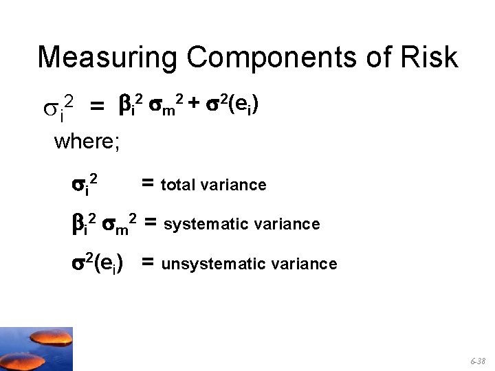
Measuring Components of Risk i 2 = bi 2 m 2 + 2(ei) where; i 2 = total variance bi 2 m 2 = systematic variance 2(ei) = unsystematic variance 6 -38

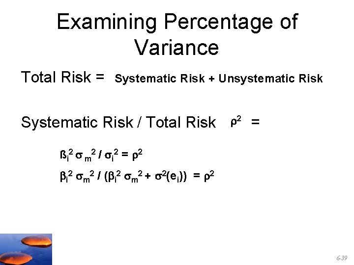
Examining Percentage of Variance Total Risk = Systematic Risk + Unsystematic Risk Systematic Risk / Total Risk 2 = ßi 2 m 2 / i 2 = 2 bi 2 m 2 / (bi 2 m 2 + 2(ei)) = 2 6 -39

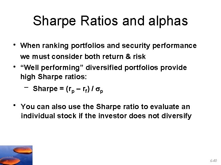
Sharpe Ratios and alphas • When ranking portfolios and security performance we must consider both return & risk • “Well performing” diversified portfolios provide high Sharpe ratios: – Sharpe = (rp – rf) / p • You can also use the Sharpe ratio to evaluate an individual stock if the investor does not diversify 6 -40

Sharpe Ratios and alphas • “Well performing” individual stocks held in diversified portfolios can be evaluated by the stock’s alpha in relation to the stock’s unsystematic risk. 6 -41