Chapter 11 Monopoly Defining Monopoly a market structure

Chapter 11 Monopoly

Defining Monopoly: a market structure in which a single seller of a product with no close substitutes serves the entire market. The key feature that differentiates the monopoly from the competitive firm is the price elasticity of demand facing the firm. For the perfectly competitive firm, recall, price elasticity is infinite. If a competitive firm raises its price only slightly, it will lose all its sales. A monopoly, by contrast, has significant control over the price it charges. The important distinction between monopoly and competition is that the demand curve facing the individual competitive firm is horizontal (irrespective of the price elasticity of the corresponding market demand curve), while the monopolist’s demand curve is simply the downward-sloping demand curve for the entire market. © 2015 Mc. Graw-Hill Education. All Rights Reserved. 2

Very stringent requirements for pure monopoly: 1. Only one firm in industry. 2. No close substitutes for the good firm produces. 3. Some reason why entry and survival of a competing firm is unlikely. • Pure monopolies are rare in real world because most firms face competition from firms producing substitutes. – E. g. , sole provider of natural gas in a city is not a pure monopoly, since other firms provide substitutes like heating oil and electricity. – E. g. , if there is only one railroad, it still competes with bus lines, trucking companies, and airlines.

The key difference: A monopoly firm has market power, the ability to influence the market price of the product it sells. A competitive firm has no market power. © 2015 Mc. Graw-Hill Education. All Rights Reserved. 4

The main cause of monopolies is barriers to entry – other firms cannot enter the market. Five sources of barriers to entry: Five Sources Of Monopoly 1. 2. 3. 4. 5. Exclusive Control over Important Inputs Economies of Scale Patents Network Economies Government Licenses or Franchises © 2015 Mc. Graw-Hill Education. All Rights Reserved. 5

1. Exclusive Control over Important Inputs The Perrier Corporation of France sells bottled mineral water. It spends millions of dollars each year advertising the unique properties of this water, which are the result, it says, of a once-in-eternity union of geological factors that created their mineral spring. In New York State, the Adirondack Soft Drink Company offers a product that is essentially tap water saturated with carbon dioxide gas. I am unable to tell the difference between Adirondack Seltzer and Perrier. But others feel differently, and for many of them there is simply no satisfactory substitute for Perrier’s monopoly position with respect to these buyers is the result of its exclusive control over an input that cannot easily be duplicated. © 2015 Mc. Graw-Hill Education. All Rights Reserved. 6

A similar monopoly position has resulted from the de. Beers Diamond Mines’ exclusive control over most of the world’s supply of raw diamonds. Synthetic diamonds have now risen in quality to the point where they can occasionally fool even an experienced jeweler. But for many buyers, the preference for a stone that was mined from the earth is not a simple matter of greater hardness and refractive brilliance. They want real diamonds, and de. Beers is the company that has them. © 2015 Mc. Graw-Hill Education. All Rights Reserved. 7

Exclusive control of key inputs is not a guarantee of permanent monopoly power. The preference for having a real diamond, for example, is based largely on the fact that mined diamonds have historically been genuinely superior to synthetic ones. But assuming that synthetic diamonds eventually do become completely indistinguishable from real ones, there will no longer be any basis for this preference. And as a result, de. Beers’ control over the supply of mined diamonds will cease to confer monopoly power. New ways are constantly being devised of producing existing products, and the exclusive input that generates today’s monopoly is likely to become obsolete tomorrow. © 2015 Mc. Graw-Hill Education. All Rights Reserved. 8

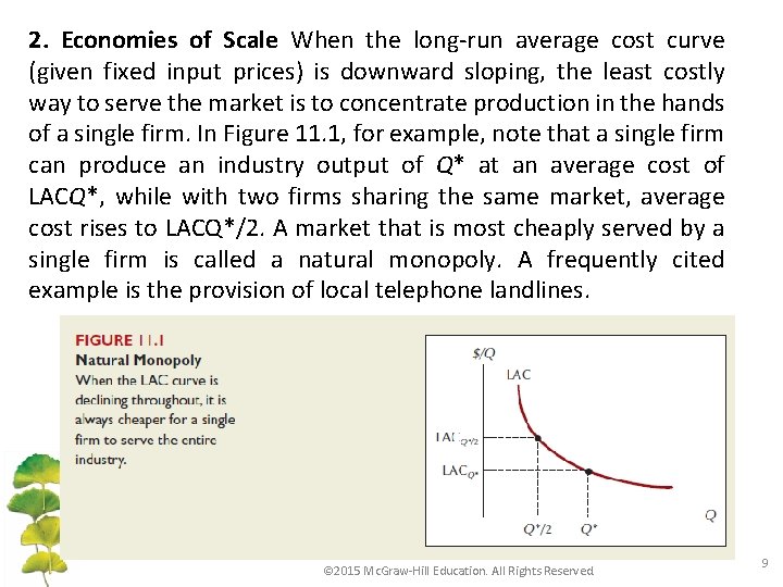
2. Economies of Scale When the long-run average cost curve (given fixed input prices) is downward sloping, the least costly way to serve the market is to concentrate production in the hands of a single firm. In Figure 11. 1, for example, note that a single firm can produce an industry output of Q* at an average cost of LACQ*, while with two firms sharing the same market, average cost rises to LACQ*/2. A market that is most cheaply served by a single firm is called a natural monopoly. A frequently cited example is the provision of local telephone landlines. © 2015 Mc. Graw-Hill Education. All Rights Reserved. 9

3. Patents Most countries protect inventions through some sort of patent system. A patent typically talks the right to exclusive benefit from all exchanges involving the invention to which it applies. There are costs as well as benefits to patents. On the cost side, the monopoly it creates usually leads, as we will see, to higher prices for consumers. On the benefit side, the patent makes possible a great many inventions that would not otherwise occur. Although some inventions are unforeseen, most are the result of long effort and expense in sophisticated research laboratories. If a firm were unable to sell its product for a sufficiently high price to earn these outlays, it would have no economic reason to undertake research and development in the first place. © 2015 Mc. Graw-Hill Education. All Rights Reserved. 10

Without a patent, competition would force price down to marginal cost, and the pace of innovation would be slowed dramatically. The protection from competition afforded by a patent is what makes it possible for the firm to recover its costs of innovation. In the United States, the life of a patent is 17 years, a compromise figure that is too long for many inventions, too short for many others. In particular, there is a persuasive argument that the patent life should be extended in the prescription drug industry, where the testing and approval process often consumes all but a few years of the current patent period © 2015 Mc. Graw-Hill Education. All Rights Reserved. 11

4. Network Economies On the demand side of many markets, a product becomes more valuable as greater numbers of consumers use it. In extreme cases, such network economies function like economies of scale as a source of natural monopoly. Microsoft’s Windows operating system, for example, achieved its dominant market position on the strength of powerful network economies. Because Microsoft’s initial sales advantage gave software developers a strong incentive to write for the Windows format, the inventory of available software in the Windows format quickly became vastly larger than for any competing operating system. And although general-purpose software such as word processors and spreadsheets continued to be available for multiple operating systems, specialized professional software and games usually appeared first in the Windows format and often only in that format. © 2015 Mc. Graw-Hill Education. All Rights Reserved. 12

This software gap gave many people a good reason for choosing Windows, even if, as in the case of many Apple Macintosh users, they believed a competing system was otherwise superior. The end result was that at one point, more than 90 percent of the world’s personal computers ran the Microsoft’s Windows operating system. If that wasn’t a pure monopoly, it came extremely close. © 2015 Mc. Graw-Hill Education. All Rights Reserved. 13

5. Government Licenses or Franchises In many markets, the law prevents anyone but a government-licensed firm from doing business. At rest areas on the Turnpike, for example, not just any fast-food restaurant is free to set up operations. The Turnpike Authority negotiates with several companies, chooses one, and then grants it an exclusive license to serve a particular area. As someone who likes Whoppers better than Big Macs, I am happy that the Mass. Pike chose Burger King over Mc. Donald’s. But their choice is bound to disappoint many other buyers. The Turnpike’s purpose in restricting access in the first place is that there is simply not room for more than one establishment in these locations. In such cases, the government license as a source of monopoly is really a scale economy acting in another form. But government licenses are also required in a variety of other markets, such as the one for taxis, where scale economies do not seem to be an important factor. To raise revenues, many college campuses (such as Ohio State) sell exclusive rights to vending machine sales (such as only Coke or only Pepsi). © 2015 Mc. Graw-Hill Education. All Rights Reserved. 14

THE PROFIT-MAXIMIZING MONOPOLIST As in the competitive case, we assume that the monopolist’s goal is to maximize economic profit. And again as before, in the short run this means to choose the level of output for which the difference between total revenue and short-run total cost is greatest. The case for this motive is less forcing than in the case of perfect competition. After all, the monopolist’s survival is less under restriction than the competitor’s, and so the evolutionary argument for profit maximization applies with less force in the monopoly case. Nonetheless, we will explore just what behaviors follow from the monopolist’s goal of profit maximization. © 2015 Mc. Graw-Hill Education. All Rights Reserved. 15

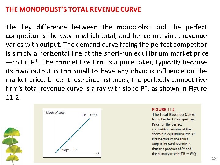
THE MONOPOLIST’S TOTAL REVENUE CURVE The key difference between the monopolist and the perfect competitor is the way in which total, and hence marginal, revenue varies with output. The demand curve facing the perfect competitor is simply a horizontal line at the short-run equilibrium market price —call it P*. The competitive firm is a price taker, typically because its own output is too small to have any obvious influence on the market price. Under these circumstances, the perfectly competitive firm’s total revenue curve is a ray with slope P*, as shown in Figure 11. 2. 16

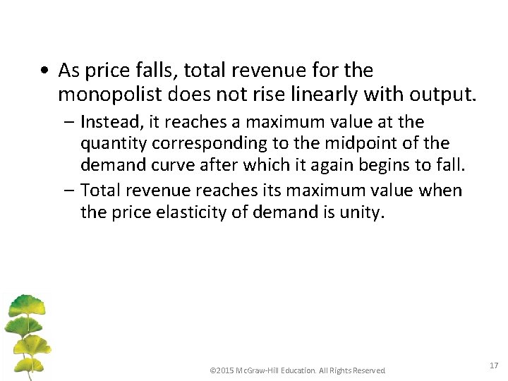
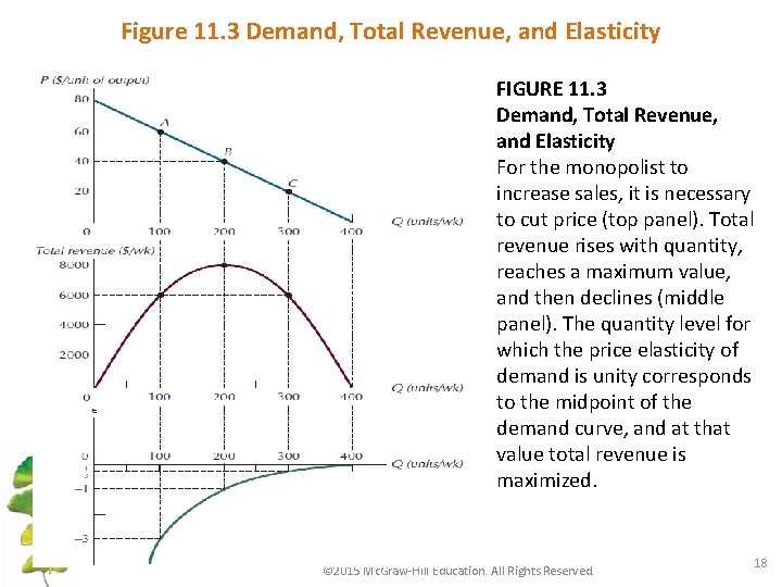
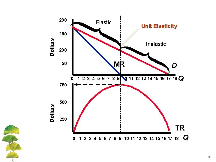
• As price falls, total revenue for the monopolist does not rise linearly with output. – Instead, it reaches a maximum value at the quantity corresponding to the midpoint of the demand curve after which it again begins to fall. – Total revenue reaches its maximum value when the price elasticity of demand is unity. © 2015 Mc. Graw-Hill Education. All Rights Reserved. 17

Figure 11. 3 Demand, Total Revenue, and Elasticity FIGURE 11. 3 Demand, Total Revenue, and Elasticity For the monopolist to increase sales, it is necessary to cut price (top panel). Total revenue rises with quantity, reaches a maximum value, and then declines (middle panel). The quantity level for which the price elasticity of demand is unity corresponds to the midpoint of the demand curve, and at that value total revenue is maximized. © 2015 Mc. Graw-Hill Education. All Rights Reserved. 18

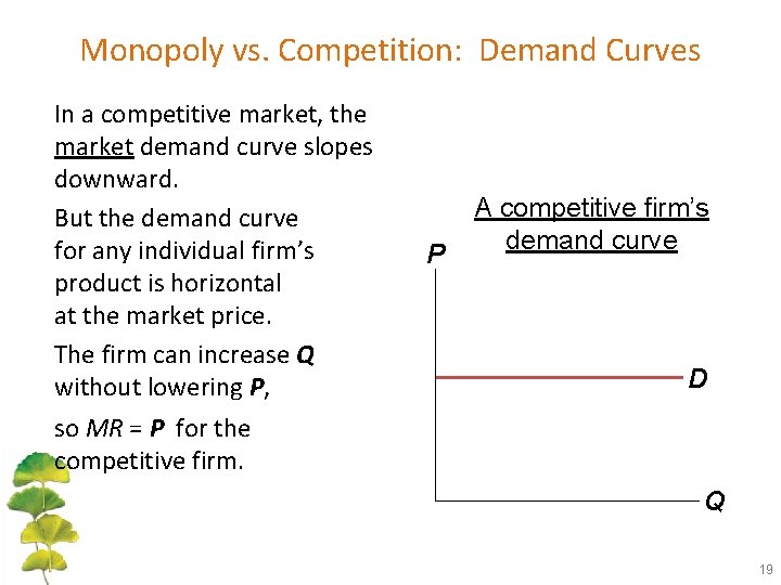
Monopoly vs. Competition: Demand Curves In a competitive market, the market demand curve slopes downward. But the demand curve for any individual firm’s product is horizontal at the market price. The firm can increase Q without lowering P, so MR = P for the competitive firm. P A competitive firm’s demand curve D Q 19

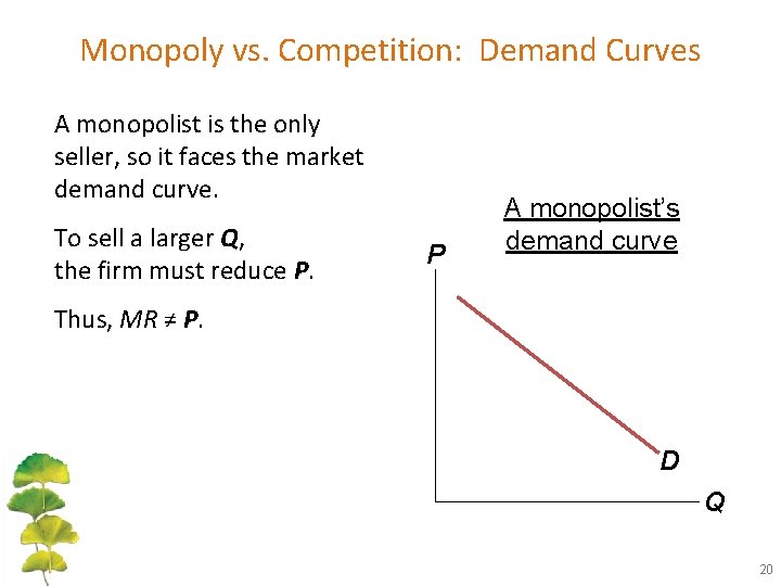
Monopoly vs. Competition: Demand Curves A monopolist is the only seller, so it faces the market demand curve. To sell a larger Q, the firm must reduce P. P A monopolist’s demand curve Thus, MR ≠ P. D Q 20

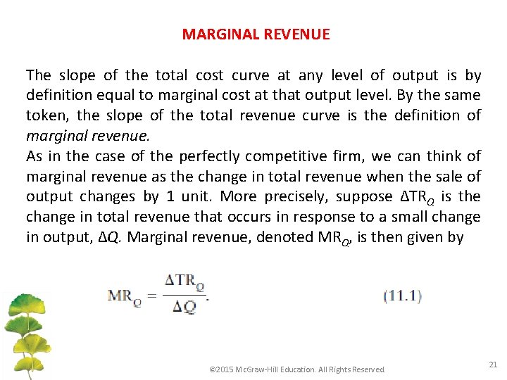
MARGINAL REVENUE The slope of the total cost curve at any level of output is by definition equal to marginal cost at that output level. By the same token, the slope of the total revenue curve is the definition of marginal revenue. As in the case of the perfectly competitive firm, we can think of marginal revenue as the change in total revenue when the sale of output changes by 1 unit. More precisely, suppose ∆TRQ is the change in total revenue that occurs in response to a small change in output, ∆Q. Marginal revenue, denoted MRQ, is then given by © 2015 Mc. Graw-Hill Education. All Rights Reserved. 21

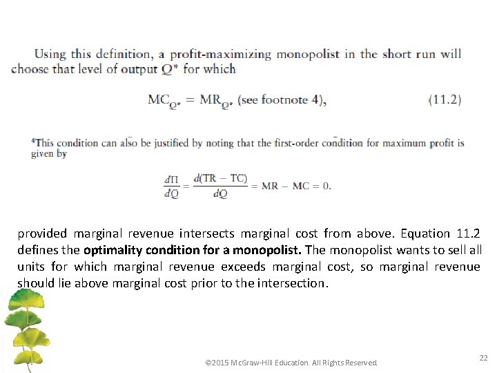
provided marginal revenue intersects marginal cost from above. Equation 11. 2 defines the optimality condition for a monopolist. The monopolist wants to sell all units for which marginal revenue exceeds marginal cost, so marginal revenue should lie above marginal cost prior to the intersection. © 2015 Mc. Graw-Hill Education. All Rights Reserved. 22

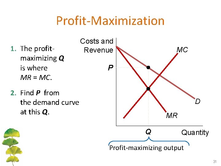
Recall that the similar condition for the perfectly competitive firm is to choose the output level for which price and marginal cost are equal. Recalling that marginal revenue and price (P) are exactly the same for the competitive firm, we see that the profit-maximizing condition for the perfectly competitive firm is simply a special case of Equation 11. 2. In the case of the monopoly firm, marginal revenue will always be less than price. Like a competitive firm, a monopolist maximizes profit by producing the quantity where MR = MC. Once the monopolist identifies this quantity, it sets the highest price consumers are willing to pay for that quantity. It finds this price from the D curve. © 2015 Mc. Graw-Hill Education. All Rights Reserved. 23

Understanding the Monopolist’s MR • Increasing Q has two effects on revenue: – Output effect: higher output raises revenue – Price effect: lower price reduces revenue • To sell a larger Q, the monopolist must reduce the price on all the units it sells. • Hence, MR < P • MR could even be negative if the price effect exceeds the output effect. • Note that a competitive firm has the output effect but not the price effect: the competitive firm does not need to reduce its price in order to sell a larger quantity, so, for the competitive firm, MR = P. MONOPOLY 24

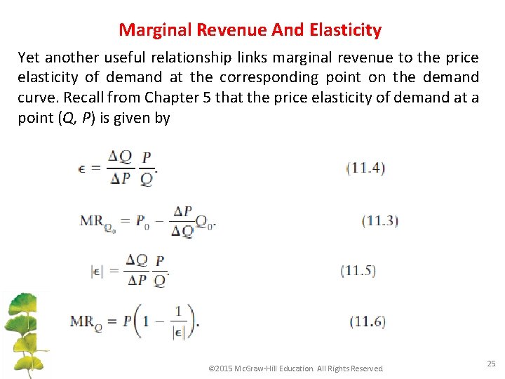
Marginal Revenue And Elasticity Yet another useful relationship links marginal revenue to the price elasticity of demand at the corresponding point on the demand curve. Recall from Chapter 5 that the price elasticity of demand at a point (Q, P) is given by © 2015 Mc. Graw-Hill Education. All Rights Reserved. 25

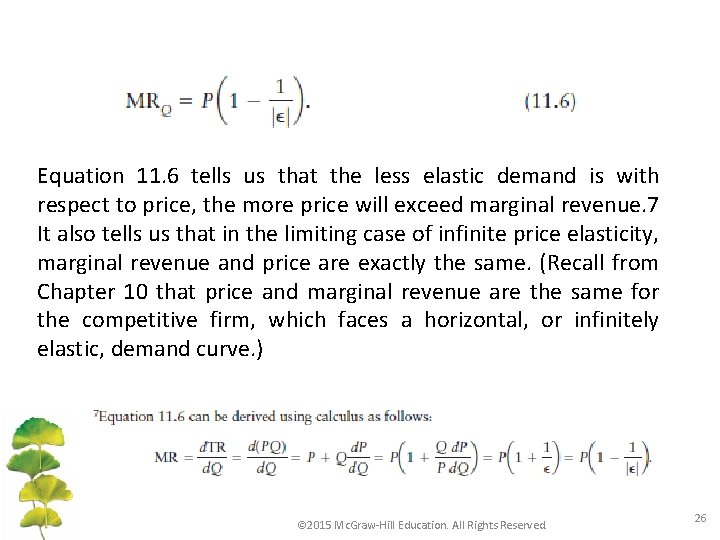
Equation 11. 6 tells us that the less elastic demand is with respect to price, the more price will exceed marginal revenue. 7 It also tells us that in the limiting case of infinite price elasticity, marginal revenue and price are exactly the same. (Recall from Chapter 10 that price and marginal revenue are the same for the competitive firm, which faces a horizontal, or infinitely elastic, demand curve. ) © 2015 Mc. Graw-Hill Education. All Rights Reserved. 26

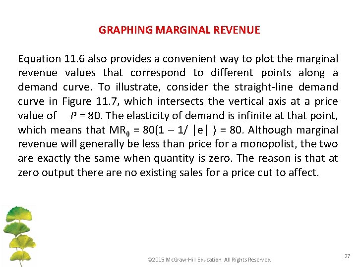
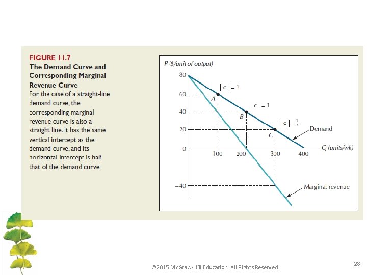
GRAPHING MARGINAL REVENUE Equation 11. 6 also provides a convenient way to plot the marginal revenue values that correspond to different points along a demand curve. To illustrate, consider the straight-line demand curve in Figure 11. 7, which intersects the vertical axis at a price value of P = 80. The elasticity of demand is infinite at that point, which means that MR 0 = 80(1 – 1/ │e│ ) = 80. Although marginal revenue will generally be less than price for a monopolist, the two are exactly the same when quantity is zero. The reason is that at zero output there are no existing sales for a price cut to affect. © 2015 Mc. Graw-Hill Education. All Rights Reserved. 27

© 2015 Mc. Graw-Hill Education. All Rights Reserved. 28

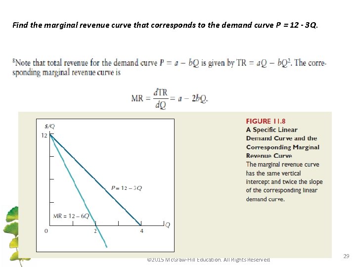
Find the marginal revenue curve that corresponds to the demand curve P = 12 - 3 Q. © 2015 Mc. Graw-Hill Education. All Rights Reserved. 29

200 Elastic Unit Elasticity Dollars 150 Inelastic 200 50 MR D 0 1 2 3 4 5 6 7 8 9 10 11 12 13 14 15 16 17 18 Dollars 750 Q 500 250 0 1 2 3 4 5 6 7 8 9 TR 10 11 12 13 14 15 16 17 18 Q 30

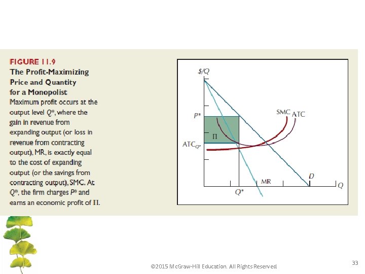
Profit-Maximization 1. The profitmaximizing Q is where MR = MC. Costs and Revenue MC P 2. Find P from the demand curve at this Q. D MR Q Quantity Profit-maximizing output 31

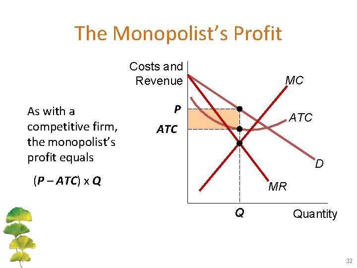
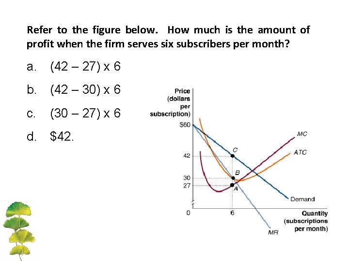
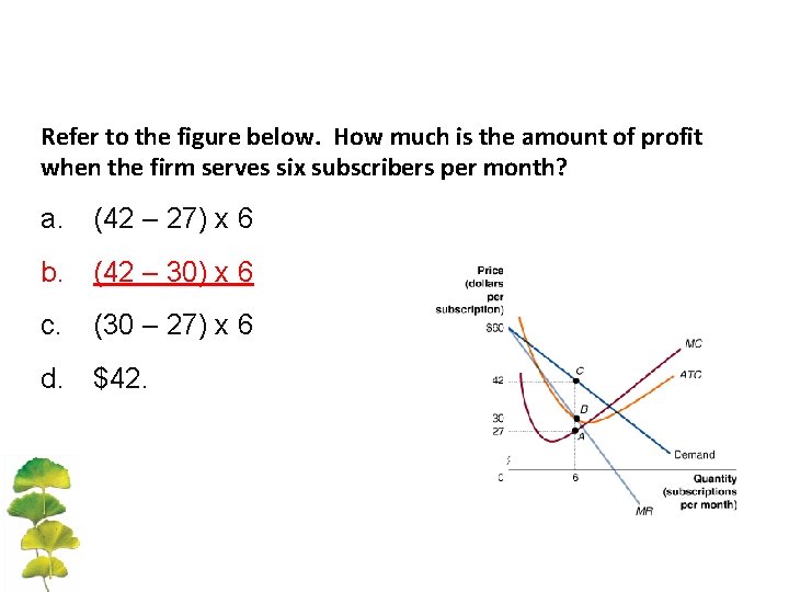
The Monopolist’s Profit Costs and Revenue As with a competitive firm, the monopolist’s profit equals MC P ATC D (P – ATC) x Q MR Q Quantity 32

© 2015 Mc. Graw-Hill Education. All Rights Reserved. 33

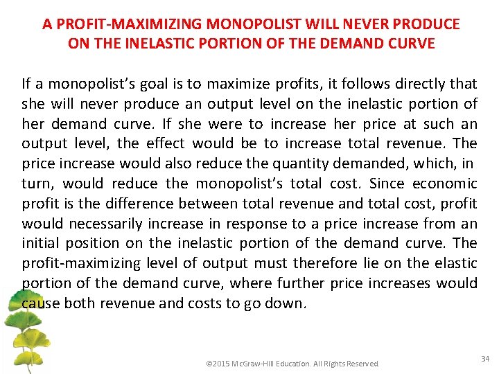
A PROFIT-MAXIMIZING MONOPOLIST WILL NEVER PRODUCE ON THE INELASTIC PORTION OF THE DEMAND CURVE If a monopolist’s goal is to maximize profits, it follows directly that she will never produce an output level on the inelastic portion of her demand curve. If she were to increase her price at such an output level, the effect would be to increase total revenue. The price increase would also reduce the quantity demanded, which, in turn, would reduce the monopolist’s total cost. Since economic profit is the difference between total revenue and total cost, profit would necessarily increase in response to a price increase from an initial position on the inelastic portion of the demand curve. The profit-maximizing level of output must therefore lie on the elastic portion of the demand curve, where further price increases would cause both revenue and costs to go down. © 2015 Mc. Graw-Hill Education. All Rights Reserved. 34

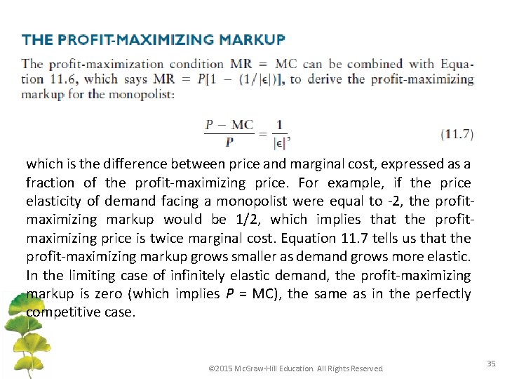
which is the difference between price and marginal cost, expressed as a fraction of the profit-maximizing price. For example, if the price elasticity of demand facing a monopolist were equal to -2, the profitmaximizing markup would be 1/2, which implies that the profitmaximizing price is twice marginal cost. Equation 11. 7 tells us that the profit-maximizing markup grows smaller as demand grows more elastic. In the limiting case of infinitely elastic demand, the profit-maximizing markup is zero (which implies P = MC), the same as in the perfectly competitive case. © 2015 Mc. Graw-Hill Education. All Rights Reserved. 35

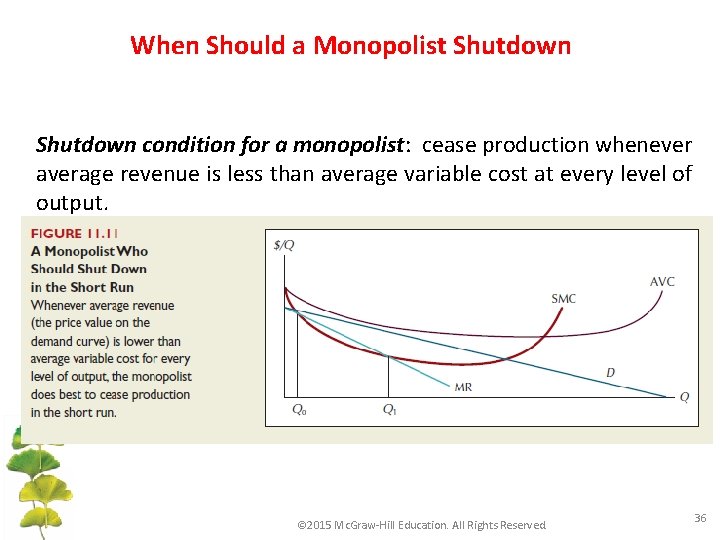
When Should a Monopolist Shutdown condition for a monopolist: cease production whenever average revenue is less than average variable cost at every level of output. © 2015 Mc. Graw-Hill Education. All Rights Reserved. 36

A Monopoly Does Not Have an S Curve A competitive firm – takes P as given – has a supply curve that shows how its Q depends on P. A monopoly firm – is a “price-maker, ” not a “price-taker” – Q does not depend on P; rather, Q and P are jointly determined by MC, MR, and the demand curve. So there is no supply curve for monopoly. 37

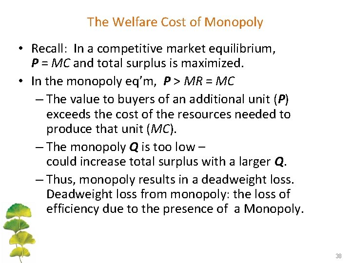
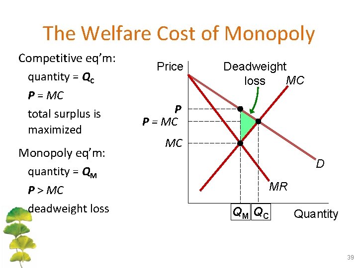
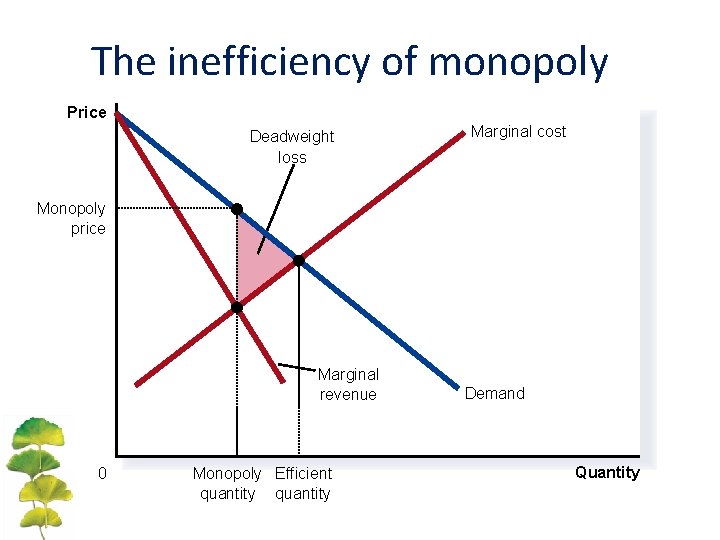
The Welfare Cost of Monopoly • Recall: In a competitive market equilibrium, P = MC and total surplus is maximized. • In the monopoly eq’m, P > MR = MC – The value to buyers of an additional unit (P) exceeds the cost of the resources needed to produce that unit (MC). – The monopoly Q is too low – could increase total surplus with a larger Q. – Thus, monopoly results in a deadweight loss. Deadweight loss from monopoly: the loss of efficiency due to the presence of a Monopoly. 38

The Welfare Cost of Monopoly Competitive eq’m: quantity = QC P = MC total surplus is maximized Monopoly eq’m: quantity = QM P > MC deadweight loss Price Deadweight MC loss P P = MC MC D MR QM QC Quantity 39

The inefficiency of monopoly Price Deadweight loss Marginal cost Monopoly price Marginal revenue 0 Monopoly Efficient quantity Demand Quantity Copyright © 2004 South-Western

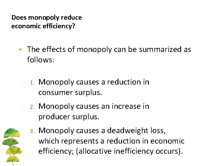
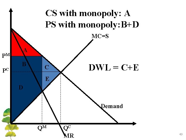
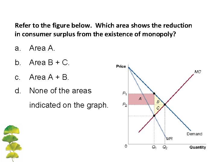
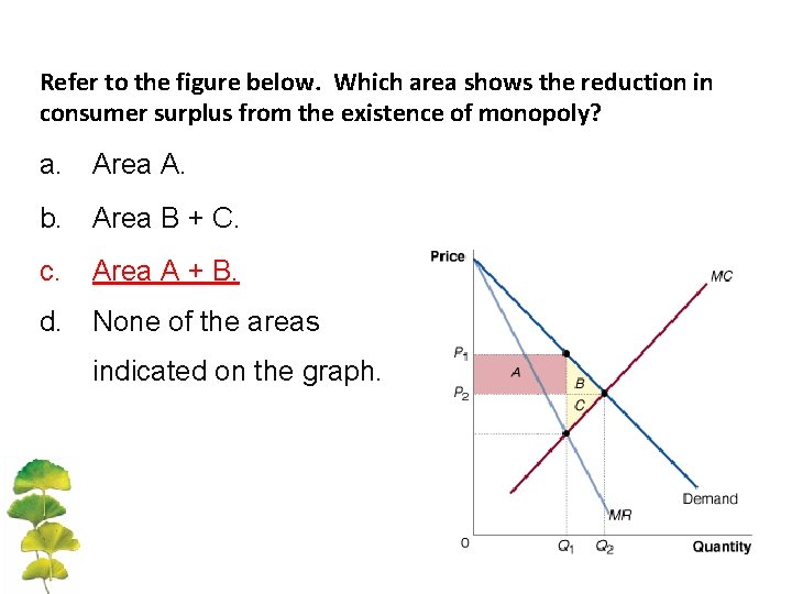
Does monopoly reduce economic efficiency? § The effects of monopoly can be summarized as follows: 1. Monopoly causes a reduction in consumer surplus. 2. Monopoly causes an increase in producer surplus. 3. Monopoly causes a deadweight loss, which represents a reduction in economic efficiency; (allocative inefficiency occurs).

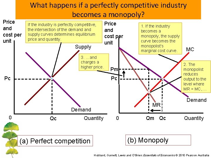
Price and cost per unit What happens if a perfectly competitive industry becomes a monopoly? If the industry is perfectly competitive, the intersection of the demand supply curves determines equilibrium price and quantity. Supply 3. …and charges a higher price. Pc Price and cost per unit Pc Qc MR Quantity (a) Perfect competition 0 MC 2. The monopolist reduces output to the level where MR = MC, … Pm Demand 0 1. If the industry becomes a monopoly, the supply curve becomes the monopolist’s marginal cost curve. Qm Qc Demand Quantity (b) Monopoly Hubbard, Garnett, Lewis and O’Brien: Essentials of Economics © 2010 Pearson Australia

PRICE DISCRIMINATION Our discussion thus far has assumed that the monopolist sells all its output at a single price. In reality, however, monopolists often charge different prices to different buyers, a practice that is known as price discrimination. In the following sections, we analyze how the profit-maximizing monopolist behaves when it is possible to charge different prices to different buyers. When price discrimination is possible, a monopolist can transfer some of the gains from consumers into its own profits. However, we will see that not all the higher profits under price discrimination come at the expense of consumers. Efficiency is enhanced as the monopolist expands output toward the level at which demand intersects marginal cost. © 2015 Mc. Graw-Hill Education. All Rights Reserved. 43

Examples of Price Discrimination Movie tickets Discounts for seniors, students, and people who can attend during weekday afternoons. They are all more likely to have lower WTP (willingness to pay ) than people who pay full price on Friday night. Airline prices Discounts for Saturday-night stayovers help distinguish business travelers, who usually have higher WTP, from more price-sensitive leisure travelers. 44

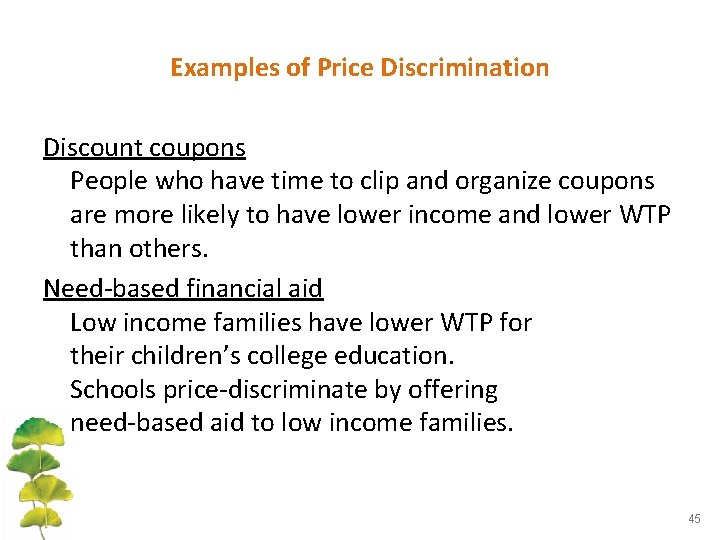
Examples of Price Discrimination Discount coupons People who have time to clip and organize coupons are more likely to have lower income and lower WTP than others. Need-based financial aid Low income families have lower WTP for their children’s college education. Schools price-discriminate by offering need-based aid to low income families. 45

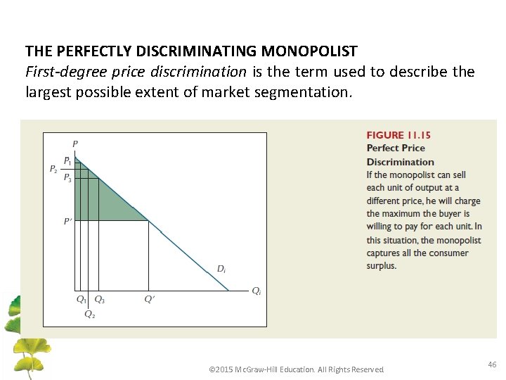
THE PERFECTLY DISCRIMINATING MONOPOLIST First-degree price discrimination is the term used to describe the largest possible extent of market segmentation. © 2015 Mc. Graw-Hill Education. All Rights Reserved. 46

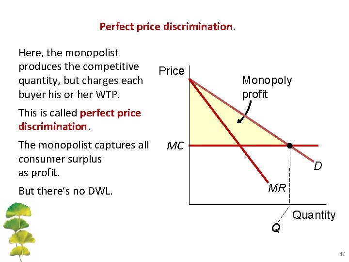
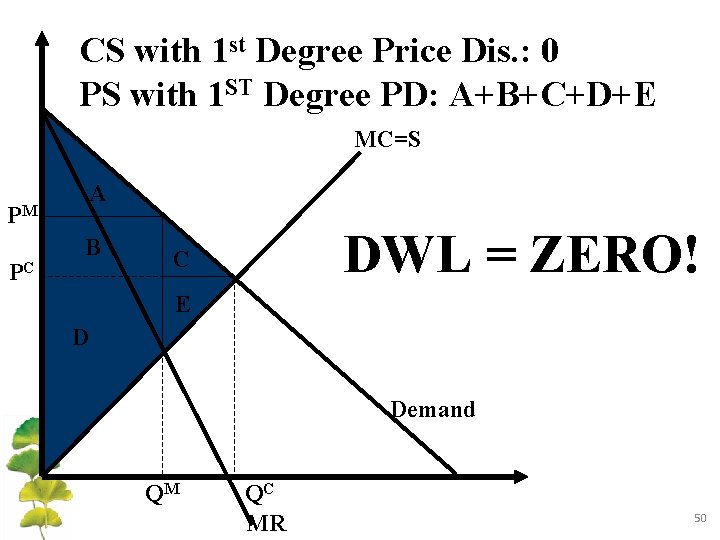
Perfect price discrimination. Here, the monopolist produces the competitive quantity, but charges each buyer his or her WTP. Price Monopoly profit This is called perfect price discrimination. The monopolist captures all consumer surplus as profit. But there’s no DWL. MC D MR Q Quantity 47

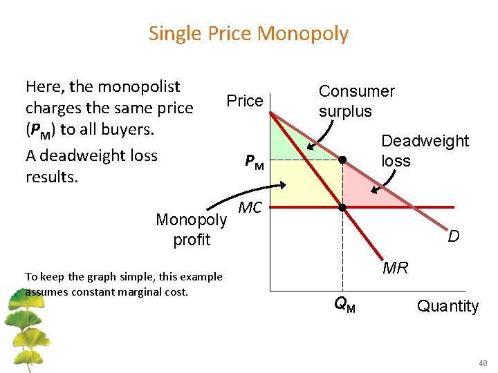
Single Price Monopoly Here, the monopolist charges the same price (PM) to all buyers. A deadweight loss results. Price Monopoly profit To keep the graph simple, this example assumes constant marginal cost. Consumer surplus Deadweight loss PM MC D MR QM Quantity 48

CS with monopoly: A PS with monopoly: B+D MC=S A PM PC B DWL = C+E C E D Demand QM QC MR 49

CS with 1 st Degree Price Dis. : 0 PS with 1 ST Degree PD: A+B+C+D+E MC=S A PM PC B DWL = ZERO! C E D Demand QM QC MR 50

Ø First Degree Price Discrimination ELIMINATES consumer surplus (each consumer pays their maximum amount) Ø First Degree Price Discrimination ELIMINATES deadweight loss (monopolists are able to provide goods to more consumers) Ø FDPD is hard to achieve and VERY weak to resale 51

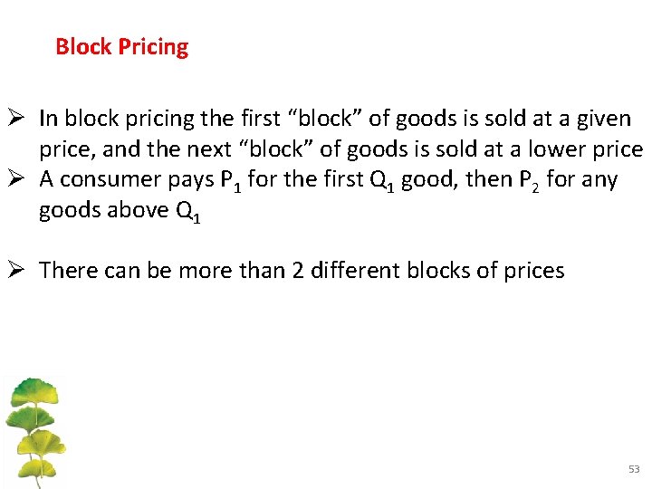
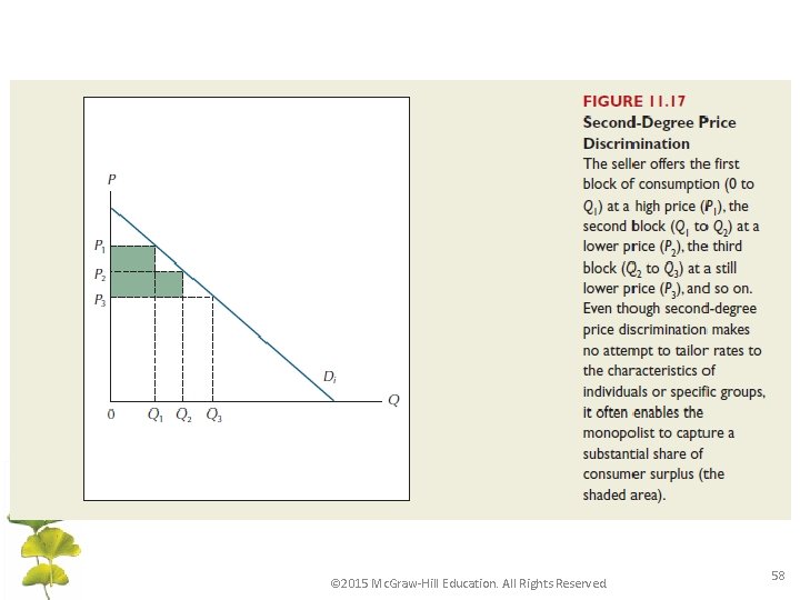
Second degree price discrimination Ø Second degree price discrimination deals with price discounts: -Selling at a discount price after a certain number of goods are purchased Ø Second degree price discrimination also involves offering separate membership and per unit price plans that consumers CHOOSE between -ie: Cell phones, club memberships, bus pass 52

Block Pricing Ø In block pricing the first “block” of goods is sold at a given price, and the next “block” of goods is sold at a lower price Ø A consumer pays P 1 for the first Q 1 good, then P 2 for any goods above Q 1 Ø There can be more than 2 different blocks of prices 53

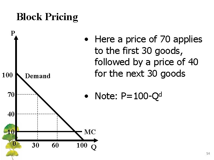
Block Pricing P 100 • Here a price of 70 applies to the first 30 goods, followed by a price of 40 for the next 30 goods Demand • Note: P=100 -Qd 70 40 10 0 MC 30 60 100 Q 54

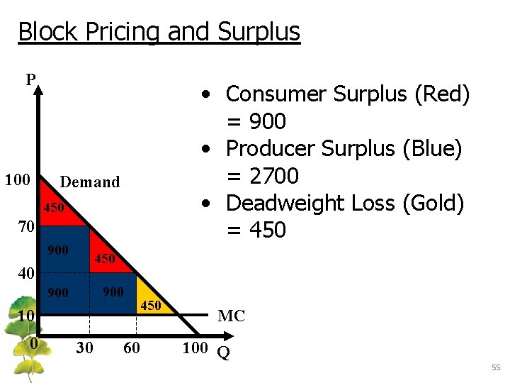
Block Pricing and Surplus P 100 • Consumer Surplus (Red) = 900 • Producer Surplus (Blue) = 2700 • Deadweight Loss (Gold) = 450 Demand 450 70 900 450 40 900 10 0 30 60 450 MC 100 Q 55

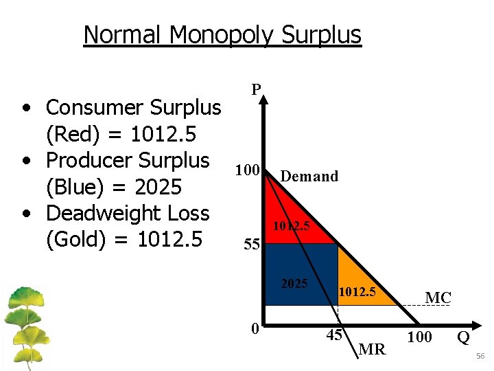
Normal Monopoly Surplus • Consumer Surplus (Red) = 1012. 5 • Producer Surplus (Blue) = 2025 • Deadweight Loss (Gold) = 1012. 5 P 100 Demand 1012. 5 55 2025 0 1012. 5 45 MR MC 100 Q 56

Ø In this example quantity discounts increased producer surplus Ø Since the quantity sold on the market also increased, DWL decreased compared to the typical monopoly Ø Note that if prices decrease due to a decreasing MC, this is not considered price discrimination 57

© 2015 Mc. Graw-Hill Education. All Rights Reserved. 58

Third degree price discrimination Ø Third degree price discrimination charges different prices to different consumer groups, or segments of society (each with different demand schedules) Ø Examples: -Student and seniors movie prices -Regular and farm gasoline -Bus passes -Tuesday deals at restaurants 59

PRICE DISCRIMINATION First Degree -Each consumer pays their maximum willingness to pay Second Degree -Consumers sort themselves into different price categories (quantity discounts or plans) Third Degree -Firms sort consumers into different price categories 60

Refer to the figure below. How much is the amount of profit when the firm serves six subscribers per month? a. (42 – 27) x 6 b. (42 – 30) x 6 c. (30 – 27) x 6 d. $42.

Refer to the figure below. How much is the amount of profit when the firm serves six subscribers per month? a. (42 – 27) x 6 b. (42 – 30) x 6 c. (30 – 27) x 6 d. $42.

Refer to the figure below. Which area shows the reduction in consumer surplus from the existence of monopoly? a. Area A. b. Area B + C. c. Area A + B. d. None of the areas indicated on the graph.

Refer to the figure below. Which area shows the reduction in consumer surplus from the existence of monopoly? a. Area A. b. Area B + C. c. Area A + B. d. None of the areas indicated on the graph.