ANOVA Experimental Design and Analysis of Variance Mc

ANOVA Experimental Design and Analysis of Variance Mc. Graw-Hill/Irwin Copyright © 2003 by The Mc. Graw-Hill Companies, Inc. All rights reserved. 10 -1 of 29

Experimental Design and Analysis of Variance 10. 1 10. 2 10. 3 10. 4 Basic Concepts of Experimental Design One-Way Analysis of Variance The Randomized Block Design Two-Way Analysis of Variance 10 -2 of 29

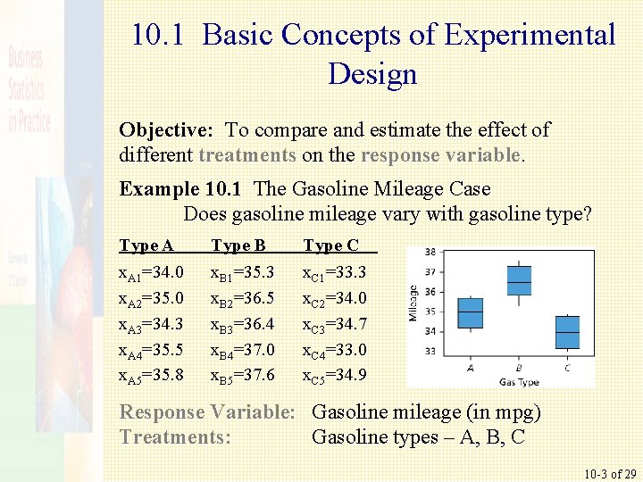
10. 1 Basic Concepts of Experimental Design Objective: To compare and estimate the effect of different treatments on the response variable. Example 10. 1 The Gasoline Mileage Case Does gasoline mileage vary with gasoline type? Type A Type B Type C x. A 1=34. 0 x. A 2=35. 0 x. A 3=34. 3 x. A 4=35. 5 x. A 5=35. 8 x. B 1=35. 3 x. B 2=36. 5 x. B 3=36. 4 x. B 4=37. 0 x. B 5=37. 6 x. C 1=33. 3 x. C 2=34. 0 x. C 3=34. 7 x. C 4=33. 0 x. C 5=34. 9 Response Variable: Gasoline mileage (in mpg) Treatments: Gasoline types – A, B, C 10 -3 of 29

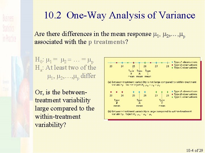
10. 2 One-Way Analysis of Variance Are there differences in the mean response m 1, m 2, …, mp associated with the p treatments? H 0: m 1 = m 2 = … = m p Ha: At least two of the m 1, m 2, …, mp differ Or, is the betweentreatment variability large compared to the within-treatment variability? 10 -4 of 29

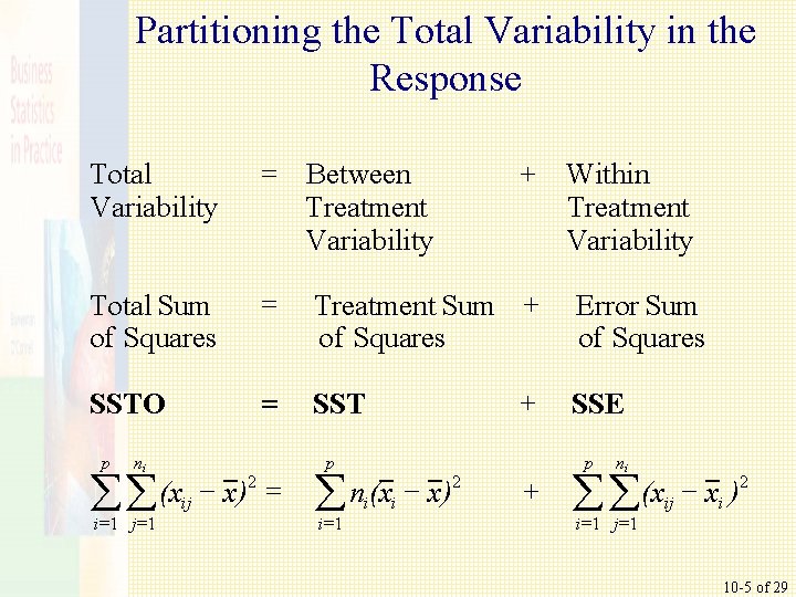
Partitioning the Total Variability in the Response Total Variability = Between Treatment Variability Total Sum of Squares = Treatment Sum + of Squares SSTO = SST p ni 2 = (x x ) åå ij i=1 j=1 p 2 n ( x x ) åi i i=1 + Within Treatment Variability + + Error Sum of Squares SSE p ni 2 (x x ) åå ij i i=1 j=1 10 -5 of 29

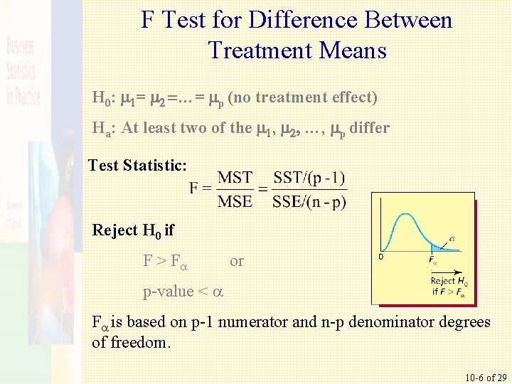
F Test for Difference Between Treatment Means H 0: m 1= m 2 =…= mp (no treatment effect) Ha: At least two of the m 1, m 2, …, mp differ Test Statistic: Reject H 0 if F > F or p-value < F is based on p-1 numerator and n-p denominator degrees of freedom. 10 -6 of 29

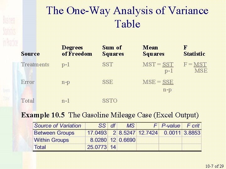
The One-Way Analysis of Variance Table Source Degrees of Freedom Sum of Squares Mean Squares F Statistic Treatments p-1 SST MST = SST p-1 F = MST MSE Error n-p SSE MSE = SSE n-p Total n-1 SSTO Example 10. 5 The Gasoline Mileage Case (Excel Output) 10 -7 of 29

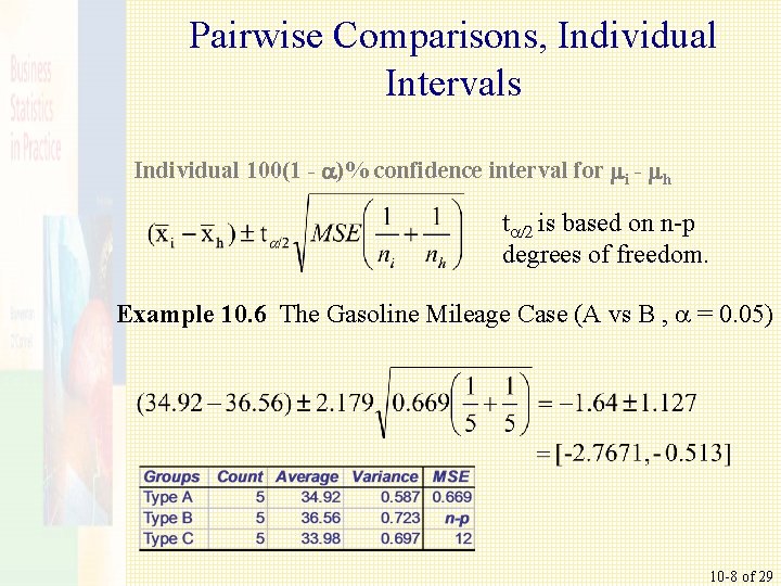
Pairwise Comparisons, Individual Intervals Individual 100(1 - a)% confidence interval for mi - mh t /2 is based on n-p degrees of freedom. Example 10. 6 The Gasoline Mileage Case (A vs B , = 0. 05) 10 -8 of 29

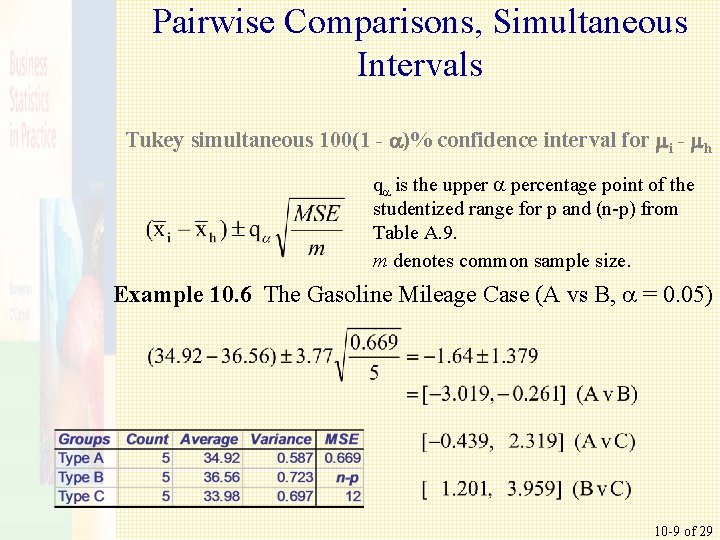
Pairwise Comparisons, Simultaneous Intervals Tukey simultaneous 100(1 - a)% confidence interval for mi - mh q is the upper percentage point of the studentized range for p and (n-p) from Table A. 9. m denotes common sample size. Example 10. 6 The Gasoline Mileage Case (A vs B, = 0. 05) 10 -9 of 29

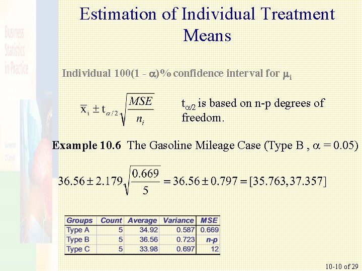
Estimation of Individual Treatment Means Individual 100(1 - a)% confidence interval for mi t /2 is based on n-p degrees of freedom. Example 10. 6 The Gasoline Mileage Case (Type B , = 0. 05) 10 -10 of 29

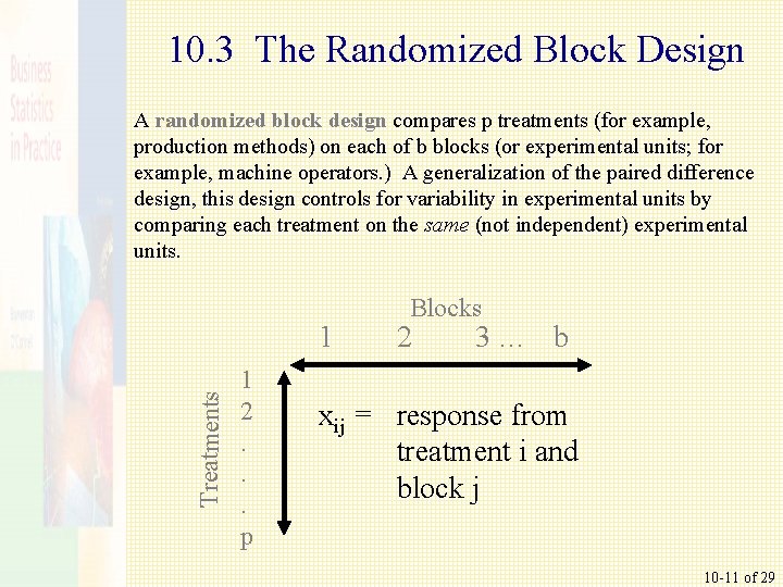
10. 3 The Randomized Block Design A randomized block design compares p treatments (for example, production methods) on each of b blocks (or experimental units; for example, machine operators. ) A generalization of the paired difference design, this design controls for variability in experimental units by comparing each treatment on the same (not independent) experimental units. Treatments 1 1 2. . . p Blocks 2 3… b xij = response from treatment i and block j 10 -11 of 29

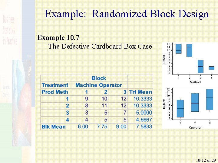
Example: Randomized Block Design Example 10. 7 The Defective Cardboard Box Case 10 -12 of 29

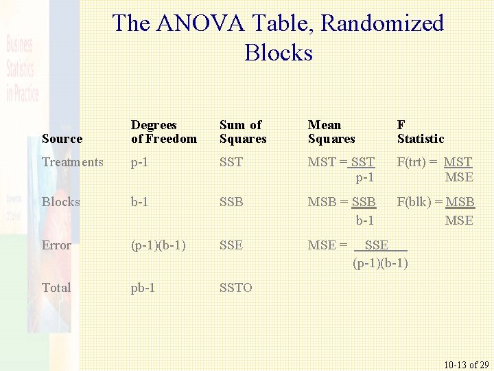
The ANOVA Table, Randomized Blocks Source Degrees of Freedom Sum of Squares Mean Squares F Statistic Treatments p-1 SST MST = SST p-1 F(trt) = MST MSE Blocks b-1 SSB MSB = SSB b-1 F(blk) = MSB MSE Error (p-1)(b-1) SSE MSE = Total pb-1 SSTO SSE (p-1)(b-1) 10 -13 of 29

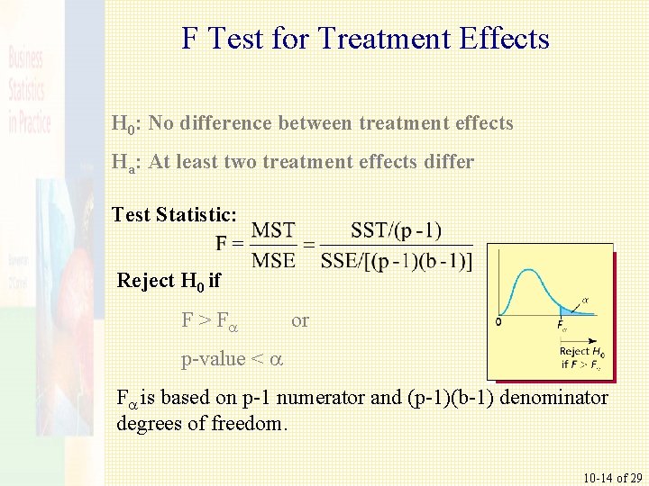
F Test for Treatment Effects H 0: No difference between treatment effects Ha: At least two treatment effects differ Test Statistic: Reject H 0 if F > F or p-value < F is based on p-1 numerator and (p-1)(b-1) denominator degrees of freedom. 10 -14 of 29

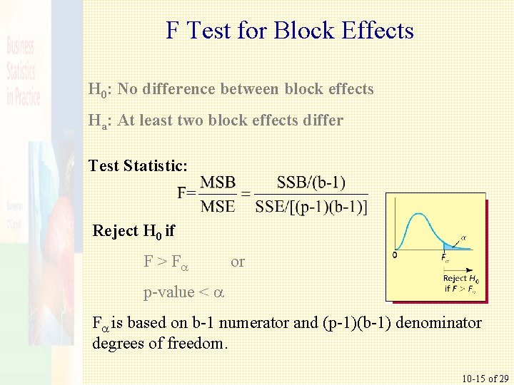
F Test for Block Effects H 0: No difference between block effects Ha: At least two block effects differ Test Statistic: Reject H 0 if F > F or p-value < F is based on b-1 numerator and (p-1)(b-1) denominator degrees of freedom. 10 -15 of 29

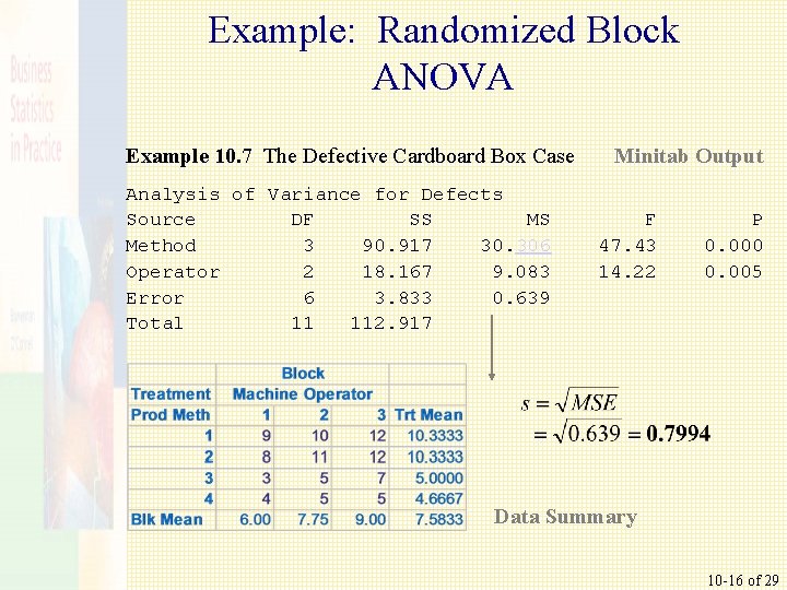
Example: Randomized Block ANOVA Example 10. 7 The Defective Cardboard Box Case Analysis of Variance for Defects Source DF SS MS Method 3 90. 917 30. 306 Operator 2 18. 167 9. 083 Error 6 3. 833 0. 639 Total 11 112. 917 Minitab Output F 47. 43 14. 22 P 0. 000 0. 005 Data Summary 10 -16 of 29

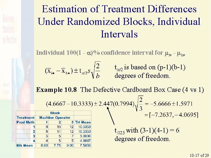
Estimation of Treatment Differences Under Randomized Blocks, Individual Intervals Individual 100(1 - a)% confidence interval for mi - mh t /2 is based on (p-1)(b-1) degrees of freedom. Example 10. 8 The Defective Cardboard Box Case (4 vs 1) t. 025 with (3 -1)(4 -1) = 6 degrees of freedom. 10 -17 of 29

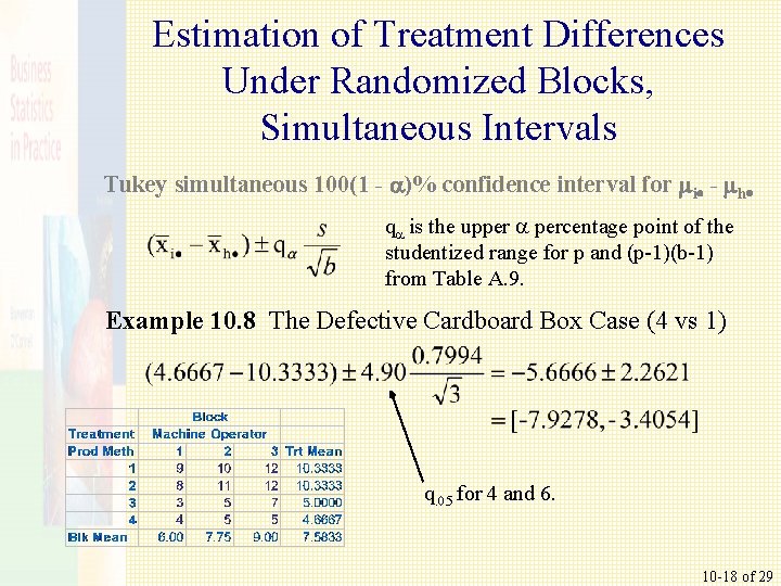
Estimation of Treatment Differences Under Randomized Blocks, Simultaneous Intervals Tukey simultaneous 100(1 - a)% confidence interval for mi - mh q is the upper percentage point of the studentized range for p and (p-1)(b-1) from Table A. 9. Example 10. 8 The Defective Cardboard Box Case (4 vs 1) q. 05 for 4 and 6. 10 -18 of 29

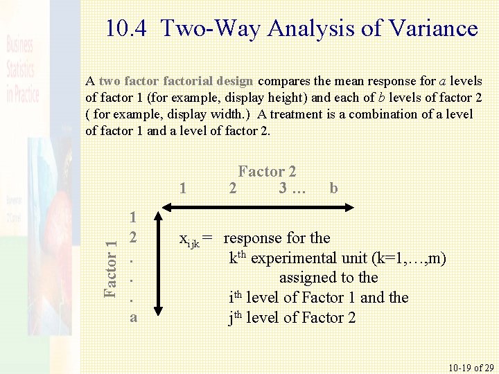
10. 4 Two-Way Analysis of Variance A two factorial design compares the mean response for a levels of factor 1 (for example, display height) and each of b levels of factor 2 ( for example, display width. ) A treatment is a combination of a level of factor 1 and a level of factor 2. Factor 1 1 1 2. . . a Factor 2 2 3… b xijk = response for the kth experimental unit (k=1, …, m) assigned to the ith level of Factor 1 and the jth level of Factor 2 10 -19 of 29

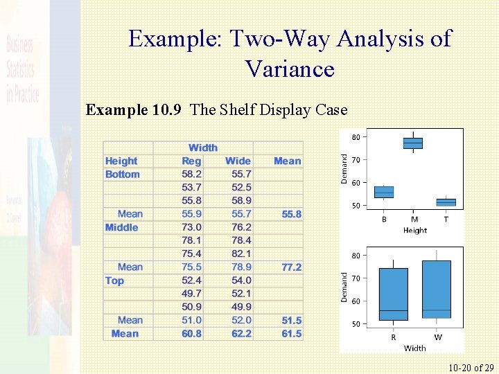
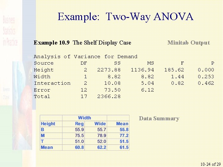
Example: Two-Way Analysis of Variance Example 10. 9 The Shelf Display Case 10 -20 of 29

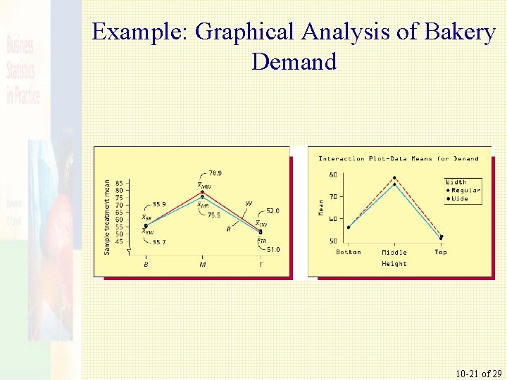
Example: Graphical Analysis of Bakery Demand 10 -21 of 29

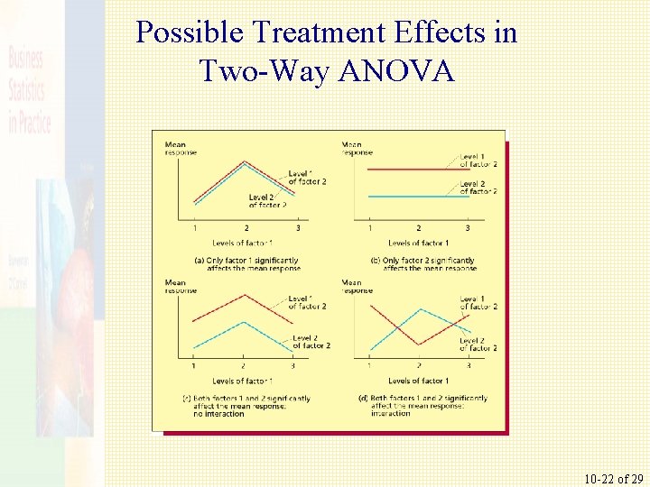
Possible Treatment Effects in Two-Way ANOVA 10 -22 of 29

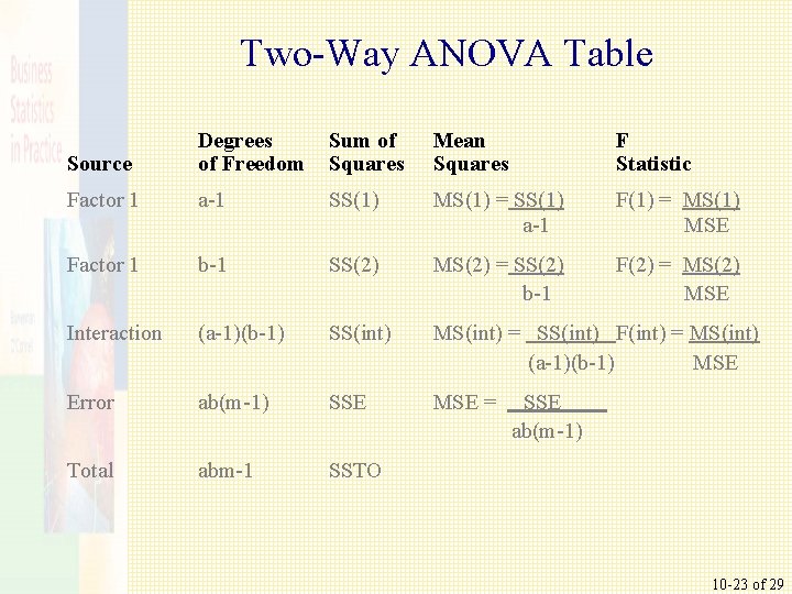
Two-Way ANOVA Table Source Degrees of Freedom Sum of Squares Mean Squares F Statistic Factor 1 a-1 SS(1) MS(1) = SS(1) a-1 F(1) = MS(1) MSE Factor 1 b-1 SS(2) MS(2) = SS(2) b-1 F(2) = MS(2) MSE Interaction (a-1)(b-1) SS(int) MS(int) = SS(int) F(int) = MS(int) (a-1)(b-1) MSE Error ab(m-1) SSE MSE = Total abm-1 SSTO SSE ab(m-1) 10 -23 of 29

Example: Two-Way ANOVA Example 10. 9 The Shelf Display Case Minitab Output Analysis of Variance for Demand Source DF SS MS Height 2 2273. 88 1136. 94 Width 1 8. 82 Interaction 2 10. 08 5. 04 Error 12 73. 50 6. 12 Total 17 2366. 28 F 185. 62 1. 44 0. 82 P 0. 000 0. 253 0. 462 Data Summary 10 -24 of 29

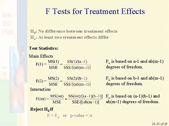
F Tests for Treatment Effects H 0: No difference between treatment effects Ha: At least two treatment effects differ Test Statistics: Main Effects F is based on a-1 and ab(m-1) degrees of freedom. F is based on b-1 and ab(m-1) degrees of freedom. Interaction F is based on (a-1)(b-1) and ab(m-1) degrees of freedom. Reject H 0 if F > F or p-value < 10 -25 of 29

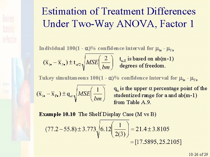
Estimation of Treatment Differences Under Two-Way ANOVA, Factor 1 Individual 100(1 - a)% confidence interval for mi - mi’ t /2 is based on ab(m-1) degrees of freedom. Tukey simultaneous 100(1 - a)% confidence interval for mi - mi’ q is the upper percentage point of the studentized range for a and ab(m-1) from Table A. 9. Example 10. 10 The Shelf Display Case (M vs B) 10 -26 of 29

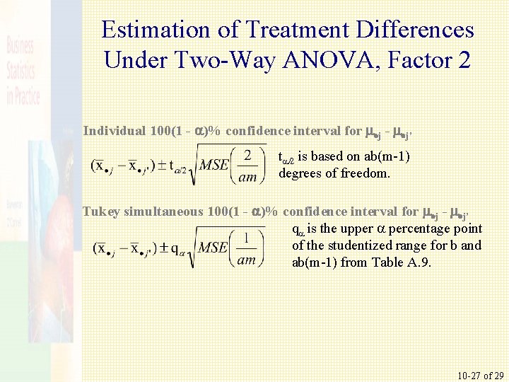
Estimation of Treatment Differences Under Two-Way ANOVA, Factor 2 Individual 100(1 - a)% confidence interval for m j - m j’ t /2 is based on ab(m-1) degrees of freedom. Tukey simultaneous 100(1 - a)% confidence interval for m j - m j’ q is the upper percentage point of the studentized range for b and ab(m-1) from Table A. 9. 10 -27 of 29

Experimental Design and Analysis of Variance 10. 1 Basic Concepts of Experimental Design Summary: 10. 2 One-Way Analysis of Variance 10. 3 The Randomized Block Design 10. 4 Two-Way Analysis of Variance 10 -28 of 29