ANALYTICAL PROPERTIES PART I ERT 207 ANALYTICAL CHEMISTRY

ANALYTICAL PROPERTIES PART I ERT 207 ANALYTICAL CHEMISTRY SEMESTER 1, ACADEMIC SESSION 2015/16

Overview 2 INTRODUCTION THE CHEMICAL METROLOGICAL HIERARCHY: UNCERTAINTY AND TRUENESS SYSTEMATIC ERRORS RANDOM ERRORS DISTRIBUTION OF EXPERIMENTAL RESULTS STATISTICAL TREATMENT OF RANDOM ERRORS bblee@unimap

Overview 3 THE SAMPLE STANDARD DEVIATION STANDARD ERROR OF THE MEAN VARIANCE AND OTHER MEASURES OF PRECISION REPORTING COMPUTED DATA bblee@unimap

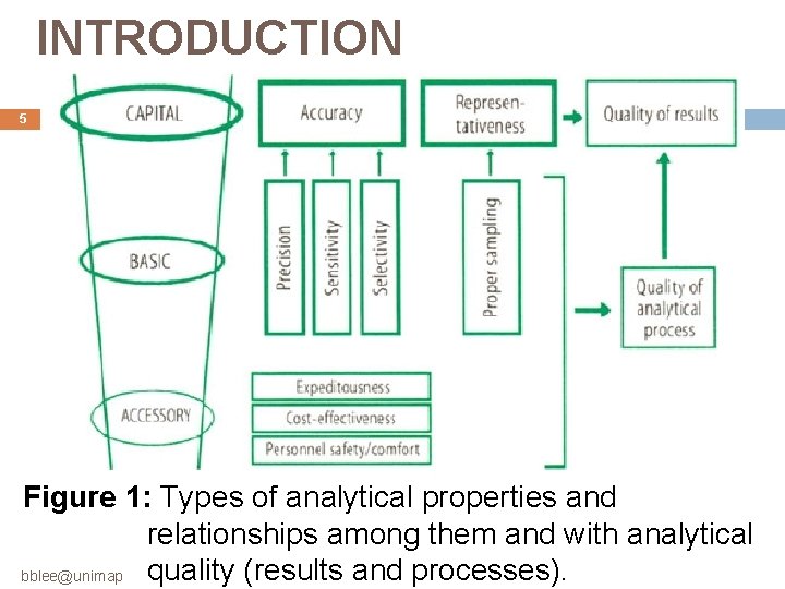
INTRODUCTION 4 Quality: Ø is defined as the totality of features (properties, attributes, capabilities) of an entity that make it equal to, better or worse than others of the same kind. Figure 1 provides an overview of analytical properties and classifies them into three hierarchical categories: Ø (i) capital properties, (ii) basic properties and bblee@unimap

INTRODUCTION 5 Figure 1: Types of analytical properties and relationships among them and with analytical quality (results and processes). bblee@unimap

INTRODUCTION 6 Capital analytical properties are typical of results (analytical information). Ø The quality of the analytical process is obviously related to that of its results; consequently, basic properties support capital properties. bblee@unimap

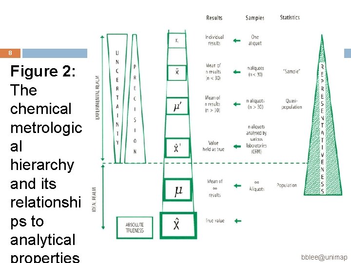
THE CHEMICAL METROLOGICAL HIERARCHY: UNCERTAINTY AND TRUENESS 7 Subjecting n aliquots of the sample to an analytical process provides n results. Ø Obviously, the quality of the information obtained will increase with increase in n. The lowest information level corresponds to an individual result (Xi) provided by a single sample aliquot. The mean obtained with n > 30, μ', will be of higher quality than the previous one. bblee@unimap

8 Figure 2: The chemical metrologic al hierarchy and its relationshi ps to analytical bblee@unimap

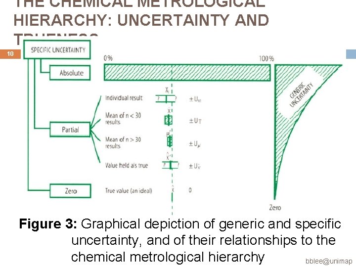
THE CHEMICAL METROLOGICAL HIERARCHY: UNCERTAINTY AND TRUENESS 9 The theoretical upper quality limit for the series being the mean for a statistical population (n = α), which is denoted by μ. When n sample aliquots are analysed by different laboratories using various analytical processes and a consensus is reached from a thorough technical study, a result X' is obtained that is held as true. Generic and specific uncertainty in Analytical Chemistry can be efficiently defined via the chemical metrological hierarchy as schematized bblee@unimap

THE CHEMICAL METROLOGICAL HIERARCHY: UNCERTAINTY AND TRUENESS 10 Figure 3: Graphical depiction of generic and specific uncertainty, and of their relationships to the chemical metrological hierarchy bblee@unimap

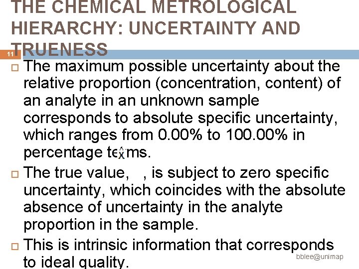
THE CHEMICAL METROLOGICAL HIERARCHY: UNCERTAINTY AND TRUENESS 11 The maximum possible uncertainty about the relative proportion (concentration, content) of an analyte in an unknown sample corresponds to absolute specific uncertainty, which ranges from 0. 00% to 100. 00% in percentage terms. The true value, , is subject to zero specific uncertainty, which coincides with the absolute absence of uncertainty in the analyte proportion in the sample. This is intrinsic information that corresponds bblee@unimap to ideal quality.

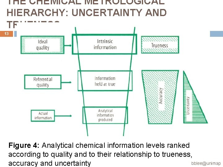
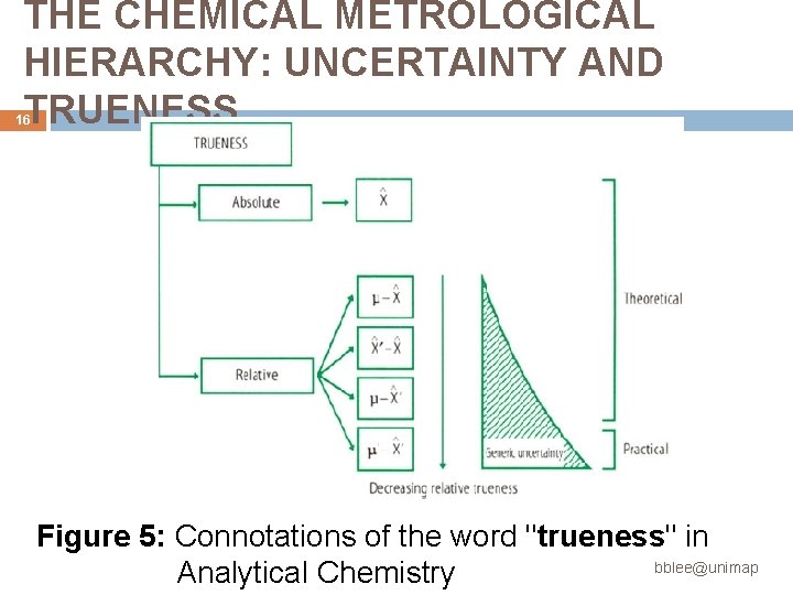
THE CHEMICAL METROLOGICAL HIERARCHY: UNCERTAINTY AND TRUENESS 12 Absolute trueness coincides with the sample's intrinsic information with the true value (X), and represents the maximum possible (ideal) quality level in Figure 4 and the top level in the metrological hierarchy of Figure 2. Figure 5 illustrates different approaches to clarify the meaning of trueness in Analytical Chemistry. bblee@unimap

THE CHEMICAL METROLOGICAL HIERARCHY: UNCERTAINTY AND TRUENESS 13 Figure 4: Analytical chemical information levels ranked according to quality and to their relationship to trueness, bblee@unimap accuracy and uncertainty

THE CHEMICAL METROLOGICAL HIERARCHY: UNCERTAINTY AND TRUENESS 14 v. Intrinsic information: Ø It is subject to no uncertainty, represents the top level of analytical quality and is characterized via an ideal, unattainable property: trueness. At a lower level is v. Referential information: Ø It is factual, reasonably accurate - nearly as much as intrinsic information - and scarcely uncertain. bblee@unimap

THE CHEMICAL METROLOGICAL HIERARCHY: UNCERTAINTY AND TRUENESS 15 Ø It is obtained under uncommon conditions (e. g. in intercomparison tests involving many participating laboratories using different analytical processes) Ø It is basically used as a reference to extract ordinary analytical information or assess its goodness. v. Actual information: Ø it is also based on facts but is less accurate and more uncertain than referential bblee@unimap

THE CHEMICAL METROLOGICAL HIERARCHY: UNCERTAINTY AND TRUENESS 16 Figure 5: Connotations of the word "trueness" in bblee@unimap Analytical Chemistry

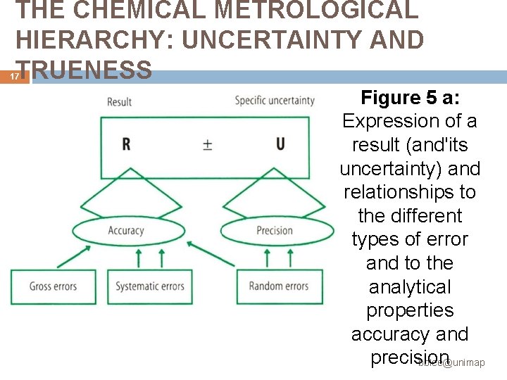
THE CHEMICAL METROLOGICAL HIERARCHY: UNCERTAINTY AND TRUENESS 17 Figure 5 a: Expression of a result (and'its uncertainty) and relationships to the different types of error and to the analytical properties accuracy and precision bblee@unimap

SYSTEMATIC ERRORS 18 Error: Ø the uncertainty in a measurement. Errors are often associated with mistakes or with something that is definitely wrong but scientists tend to think of them as either: (i) The discrepancy between a measured value and some generally accepted true value (the accuracy of the measurement), or (ii) The degree to which repeated measurement of a particular quantitybblee@unimap gives

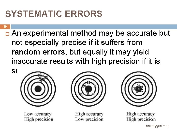
SYSTEMATIC ERRORS 19 An experimental method may be accurate but not especially precise if it suffers from random errors, but equally it may yield inaccurate results with high precision if it is subject to systematic errors. bblee@unimap

SYSTEMATIC ERRORS 20 In an experiment free from serious systematic errors, we can improve the precision considerably by increasing the sample size. Systematic errors always affect the accuracy of the result and will tend to do so in the same direction Ø the answer will always tend to be too high or too low rather than fluctuating about some central value following successive bblee@unimap

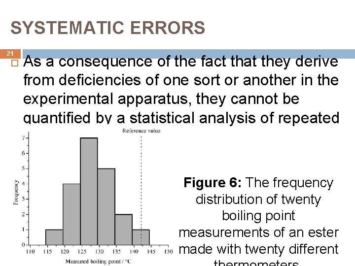
SYSTEMATIC ERRORS 21 As a consequence of the fact that they derive from deficiencies of one sort or another in the experimental apparatus, they cannot be quantified by a statistical analysis of repeated observations. Figure 6: The frequency distribution of twenty boiling point measurements of an ester made with twenty different bblee@unimap

RANDOM ERRORS 22 Random errors are present in every measurement no matter how careful the experimenter. The somewhat uncomfortable reality of experimental measurement is that two measurements of the same physical property with identical apparatus, using a nominally identical procedure, will almost invariably yield slightly different results. Repeating the measurement further will bblee@unimap

RANDOM ERRORS 23 Such variations result from random fluctuations in the experimental conditions from one measurement to the next and from limitations associated with the precision of the apparatus or the technique of whoever is conducting the experiment. The statistical nature of these fluctuations means that the discrepancies with respect to the ‘true’ value are equally likely to be positive or negative. bblee@unimap

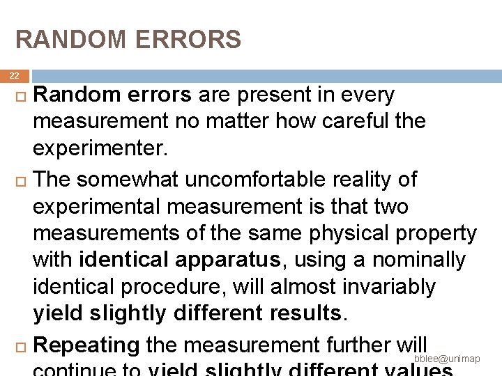
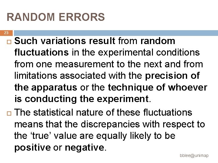
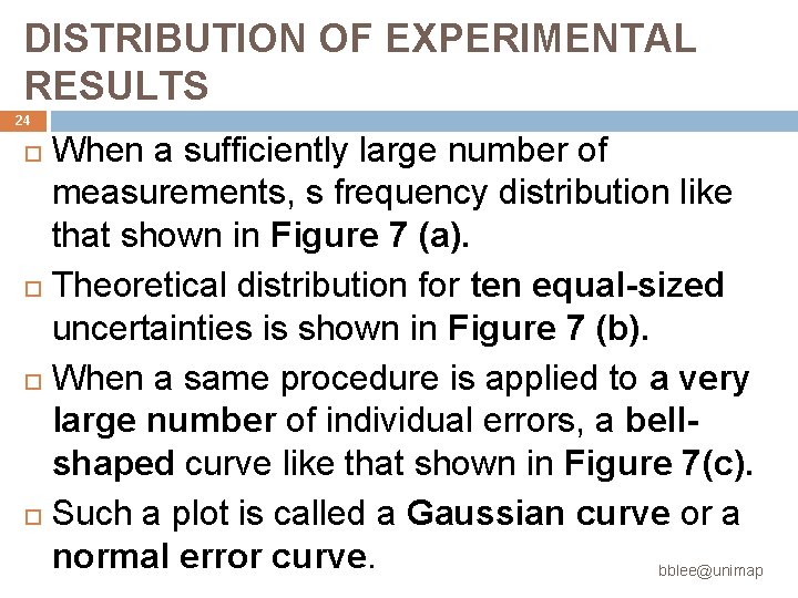
DISTRIBUTION OF EXPERIMENTAL RESULTS 24 When a sufficiently large number of measurements, s frequency distribution like that shown in Figure 7 (a). Theoretical distribution for ten equal-sized uncertainties is shown in Figure 7 (b). When a same procedure is applied to a very large number of individual errors, a bellshaped curve like that shown in Figure 7(c). Such a plot is called a Gaussian curve or a normal error curve. bblee@unimap

DISTRIBUTION OF EXPERIMENTAL RESULTS (a) 25 (b) (c) Figure 7: Frequency distribution for measurements containing (a) four random uncertainties (4 U). (b) ten random uncertainties (10 U) (c) a very large number of random uncertainties. bblee@unima

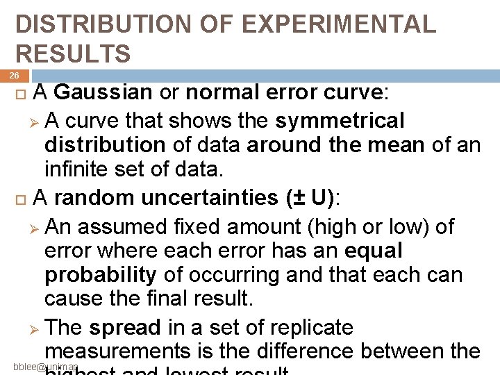
DISTRIBUTION OF EXPERIMENTAL RESULTS 26 A Gaussian or normal error curve: Ø A curve that shows the symmetrical distribution of data around the mean of an infinite set of data. A random uncertainties (± U): Ø An assumed fixed amount (high or low) of error where each error has an equal probability of occurring and that each can cause the final result. Ø The spread in a set of replicate measurements is the difference between the bblee@unimap

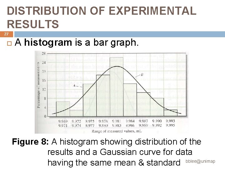
DISTRIBUTION OF EXPERIMENTAL RESULTS 27 A histogram is a bar graph. Figure 8: A histogram showing distribution of the results and a Gaussian curve for data having the same mean & standard bblee@unimap

28 STATISTICAL TREATMENT OF RANDOM ERRORS Statistical analysis: Ø Only reveals information that is already present in a data set. Ø No new information is created by statistical treatments. Statistical methods do not allow us to categorize and characterize data in different ways and to make objective and intelligent decisions about data quality and interpretation. bblee@unimap

29 STATISTICAL TREATMENT OF RANDOM ERRORS As a rule of thumb, if we have more than 30 results and the data are not heavily skewed, we can safely use a Gaussian distribution. (1) Samples and Populations We gather information about a population or universe from observation made on a subset or sample. bblee@unimap

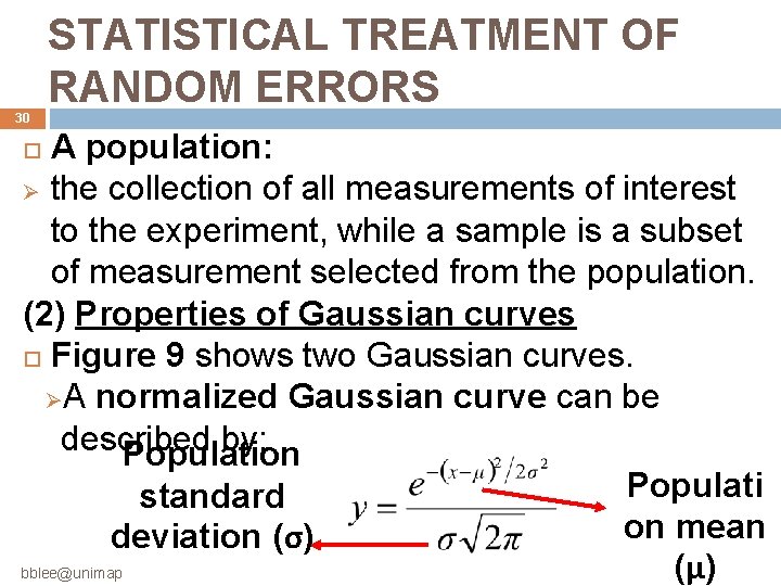
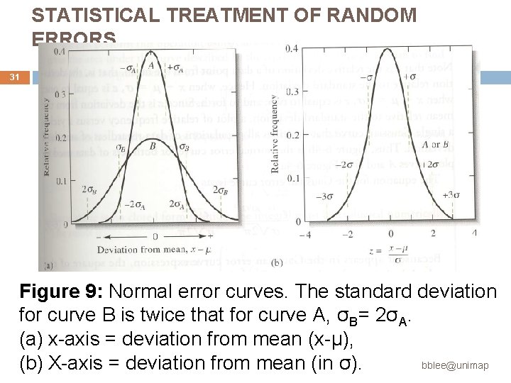
30 STATISTICAL TREATMENT OF RANDOM ERRORS A population: Ø the collection of all measurements of interest to the experiment, while a sample is a subset of measurement selected from the population. (2) Properties of Gaussian curves Figure 9 shows two Gaussian curves. ØA normalized Gaussian curve can be described by: Population Populati standard on mean deviation (σ) bblee@unimap (μ)

STATISTICAL TREATMENT OF RANDOM ERRORS 31 Figure 9: Normal error curves. The standard deviation for curve B is twice that for curve A, σB= 2σA. (a) x-axis = deviation from mean (x-μ), bblee@unimap (b) X-axis = deviation from mean (in σ).

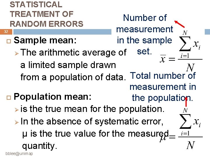
STATISTICAL TREATMENT OF RANDOM ERRORS Number of measurement in the sample Sample mean: set. Ø The arithmetic average of a limited sample drawn from a population of data. Total number of measurement in Population mean: the population. Ø is the true mean for the population. Ø In the absence of systematic error, μ is the true value for the measured quantity. 32 bblee@unimap

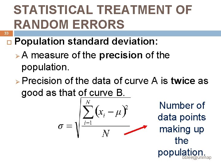
33 STATISTICAL TREATMENT OF RANDOM ERRORS Population standard deviation: Ø A measure of the precision of the population. Ø Precision of the data of curve A is twice as good as that of curve B. Number of data points making up the population. bblee@unimap

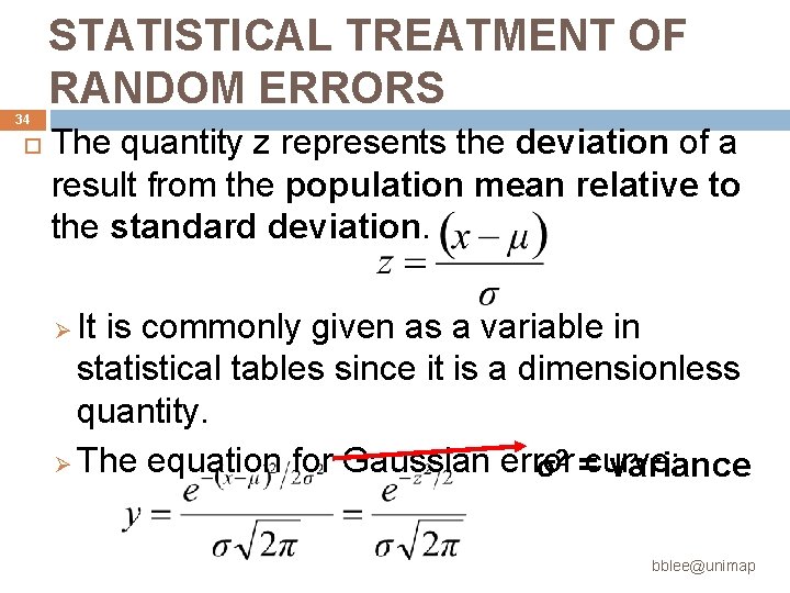
34 STATISTICAL TREATMENT OF RANDOM ERRORS The quantity z represents the deviation of a result from the population mean relative to the standard deviation. It is commonly given as a variable in statistical tables since it is a dimensionless quantity. Ø The equation for Gaussian error σ2 =curve: variance Ø bblee@unimap

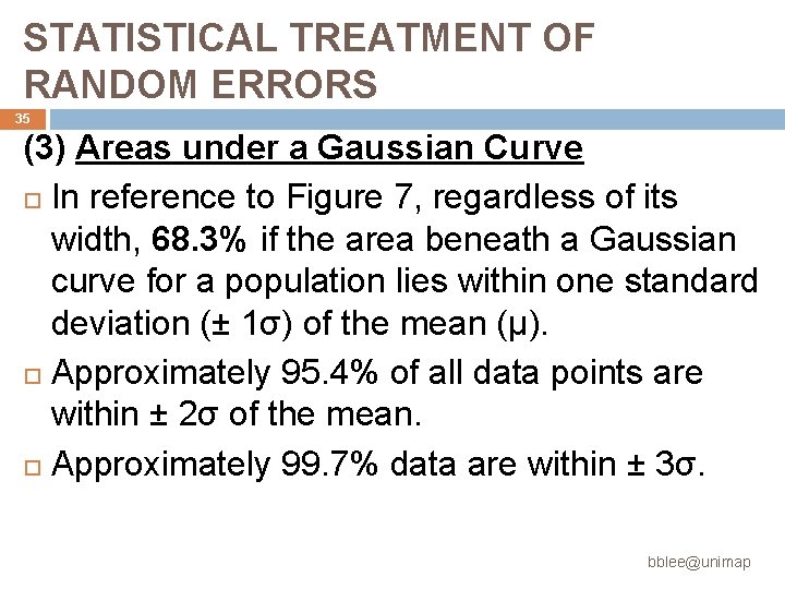
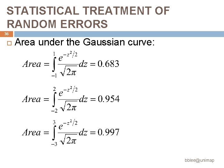
STATISTICAL TREATMENT OF RANDOM ERRORS 35 (3) Areas under a Gaussian Curve In reference to Figure 7, regardless of its width, 68. 3% if the area beneath a Gaussian curve for a population lies within one standard deviation (± 1σ) of the mean (μ). Approximately 95. 4% of all data points are within ± 2σ of the mean. Approximately 99. 7% data are within ± 3σ. bblee@unimap

STATISTICAL TREATMENT OF RANDOM ERRORS 36 Area under the Gaussian curve: bblee@unimap

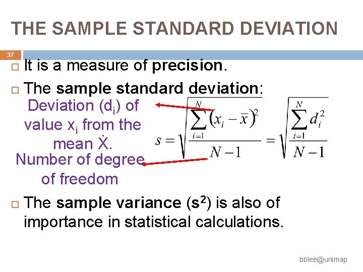
THE SAMPLE STANDARD DEVIATION 37 It is a measure of precision. The sample standard deviation: Deviation (di) of value xi from the mean Ẋ. Number of degree of freedom The sample variance (s 2) is also of importance in statistical calculations. bblee@unimap

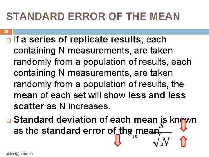
STANDARD ERROR OF THE MEAN 38 If a series of replicate results, each containing N measurements, are taken randomly from a population of results, the mean of each set will show less and less scatter as N increases. Standard deviation of each mean is known as the standard error of the mean. bblee@unimap

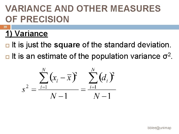
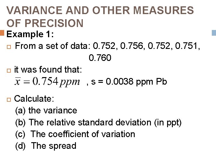
VARIANCE AND OTHER MEASURES OF PRECISION 39 1) Variance It is just the square of the standard deviation. It is an estimate of the population variance σ2. bblee@unimap

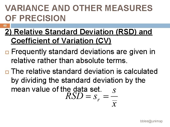
VARIANCE AND OTHER MEASURES OF PRECISION 40 2) Relative Standard Deviation (RSD) and Coefficient of Variation (CV) Frequently standard deviations are given in relative rather than absolute terms. The relative standard deviation is calculated by dividing the standard deviation by the mean value of the data set. bblee@unimap

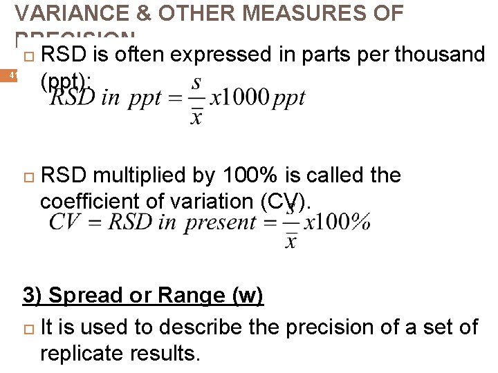
VARIANCE & OTHER MEASURES OF PRECISION RSD is often expressed in parts per thousand (ppt): 41 RSD multiplied by 100% is called the coefficient of variation (CV). 3) Spread or Range (w) It is used to describe the precision of a set of bblee@unimap replicate results.

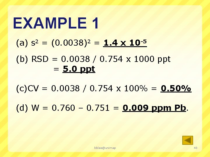
VARIANCE AND OTHER MEASURES OF PRECISION Example 1: From a set of data: 0. 752, 0. 756, 0. 752, 0. 751, 0. 760 it was found that: , s = 0. 0038 ppm Pb 42 Calculate: (a) the variance (b) The relative standard deviation (in ppt) (c) The coefficient of variation (d) The spread bblee@unimap

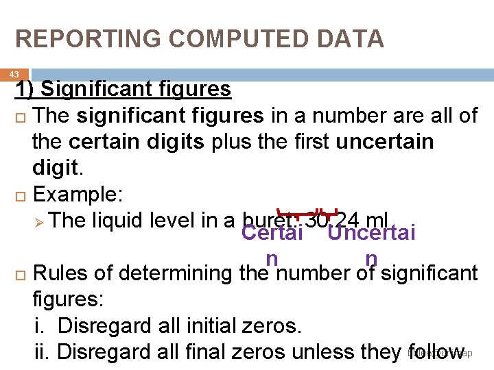
REPORTING COMPUTED DATA 43 1) Significant figures The significant figures in a number are all of the certain digits plus the first uncertain digit. Example: Ø The liquid level in a buret: 30. 24 ml Certai Uncertai n n Rules of determining the number of significant figures: i. Disregard all initial zeros. ii. Disregard all final zeros unless they bblee@unimap follow

REPORTING COMPUTED DATA 44 iii. All remaining digits including zeros between nonzero digits are significant. 2) Significant figures in numerical computations For addition & subtraction, the result should contain the same number of decimal places as the number with the smallest number of decimal places. bblee@unimap

REPORTING COMPUTED DATA 45 For multiplication and division is the number with the smallest number of significant figures. For logarithms and antilogarithms: (i) In a logarithm of a number, keep as many digits to the right of the decimal point as there are significant figures in the original number. (ii) In an antilogarithm of a number, keep as many digits as there are digits to bblee@unimap the

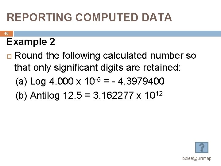
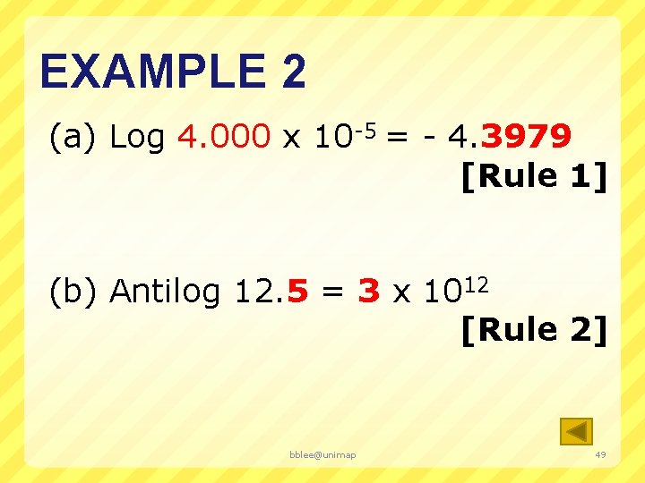
REPORTING COMPUTED DATA 46 Example 2 Round the following calculated number so that only significant digits are retained: (a) Log 4. 000 x 10 -5 = - 4. 3979400 (b) Antilog 12. 5 = 3. 162277 x 1012 bblee@unimap

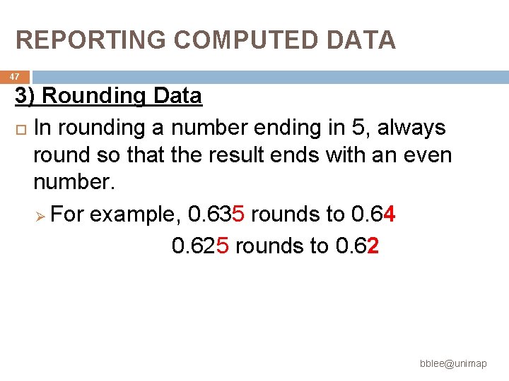
REPORTING COMPUTED DATA 47 3) Rounding Data In rounding a number ending in 5, always round so that the result ends with an even number. Ø For example, 0. 635 rounds to 0. 64 0. 625 rounds to 0. 62 bblee@unimap

EXAMPLE 1 (a) s 2 = (0. 0038)2 = 1. 4 x 10 -5 (b) RSD = 0. 0038 / 0. 754 x 1000 ppt = 5. 0 ppt (c)CV = 0. 0038 / 0. 754 x 100% = 0. 50% (d) W = 0. 760 – 0. 751 = 0. 009 ppm Pb. bblee@unimap 48

EXAMPLE 2 (a) Log 4. 000 x 10 -5 = - 4. 3979 [Rule 1] (b) Antilog 12. 5 = 3 x 1012 [Rule 2] bblee@unimap 49