Aggregate Scheduling 13 Power Point presentation to accompany

Aggregate Scheduling 13 Power. Point presentation to accompany Heizer and Render Operations Management, Global Edition, Eleventh Edition Principles of Operations Management, Global Edition, Ninth Edition Power. Point slides by Jeff Heyl © 2014 Pearson Education 13 - 1

Outline u Aggregate Planning - 0 bjective - Planning Horizon u Aggregate Planning Strategies u Capacity Options u Demand Options u Mixing Options to Develop a Plan © 2011 Pearson Education, Inc. publishing as Prentice Hall 13 - 2

Outline – Continued u Methods for Aggregate Planning u Chase Strategy u Level Strategy u Mixed Strategies u Aggregate Planning in Services © 2011 Pearson Education, Inc. publishing as Prentice Hall 13 - 3

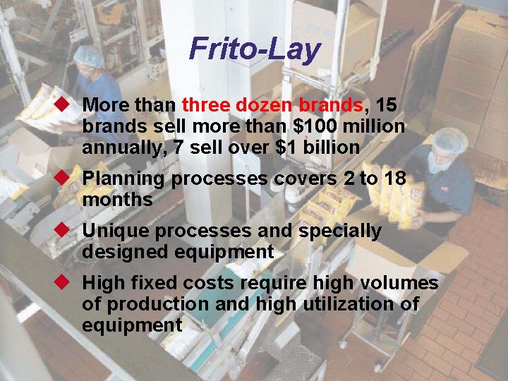
Frito-Lay u More than three dozen brands, 15 brands sell more than $100 million annually, 7 sell over $1 billion u Planning processes covers 2 to 18 months u Unique processes and specially designed equipment u High fixed costs require high volumes of production and high utilization of equipment © 2011 Pearson Education, Inc. publishing as Prentice Hall 13 - 4

Aggregate Planning The objective of aggregate planning is to meet the forecasted demand while minimizing the total cost over the planning period © 2011 Pearson Education, Inc. publishing as Prentice Hall 13 - 5

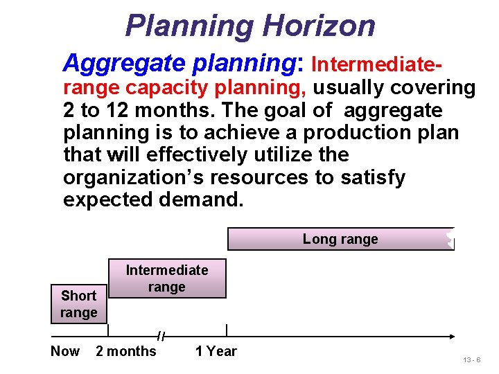
Planning Horizon Aggregate planning: Intermediate- range capacity planning, usually covering 2 to 12 months. The goal of aggregate planning is to achieve a production plan that will effectively utilize the organization’s resources to satisfy expected demand. Long range Short range Now Intermediate range 2 months 1 Year 13 - 6

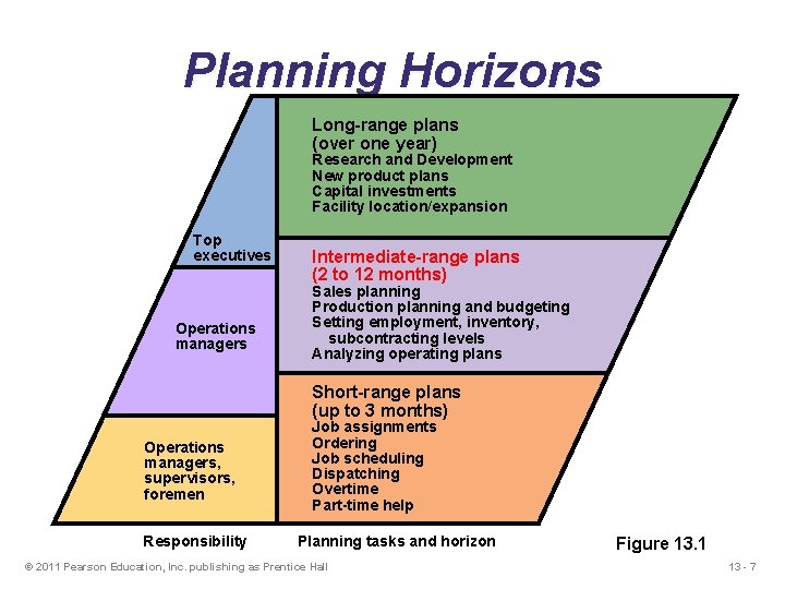
Planning Horizons Long-range plans (over one year) Research and Development New product plans Capital investments Facility location/expansion Top executives Operations managers Intermediate-range plans (2 to 12 months) Sales planning Production planning and budgeting Setting employment, inventory, subcontracting levels Analyzing operating plans Short-range plans (up to 3 months) Operations managers, supervisors, foremen Responsibility Job assignments Ordering Job scheduling Dispatching Overtime Part-time help Planning tasks and horizon © 2011 Pearson Education, Inc. publishing as Prentice Hall Figure 13. 1 13 - 7

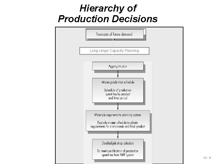
Hierarchy of Production Decisions Long-range Capacity Planning 13 - 8

Aggregate Planning u Aggregate planning is a big picture approach to production planning. u It is a production plan to meet the demand throughout the year. u It is not concerned with individual products, but with a single aggregate product representing all products. u For example, in a TV manufacturing plant, the aggregate planning does not go into all models and sizes. It only deals with a single representative aggregate TV. u All models are lumped together and represent a single product; hence the term aggregate planning is used. 13 - 9

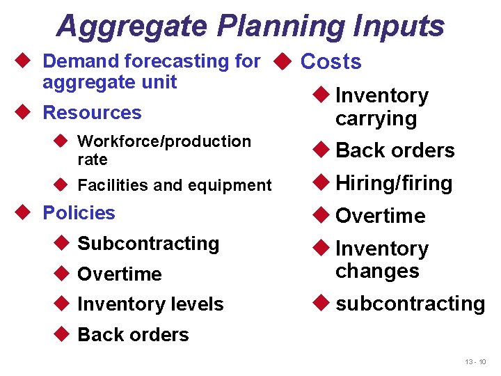
Aggregate Planning Inputs u Demand forecasting for u Costs aggregate unit u Resources u Inventory carrying u Workforce/production rate u Back orders u Facilities and equipment u Hiring/firing u Policies u Subcontracting u Overtime u Inventory changes u Inventory levels u subcontracting u Back orders 13 - 10

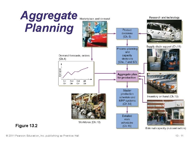
Aggregate Planning Figure 13. 2 © 2011 Pearson Education, Inc. publishing as Prentice Hall 13 - 11

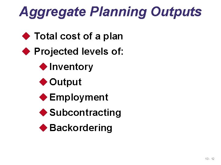
Aggregate Planning Outputs u Total cost of a plan u Projected levels of: u Inventory u Output u Employment u Subcontracting u Backordering 13 - 12

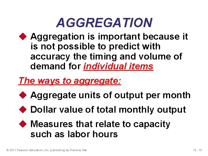
AGGREGATION u Aggregation is important because it is not possible to predict with accuracy the timing and volume of demand for individual items The ways to aggregate: u Aggregate units of output per month u Dollar value of total monthly output u Measures that relate to capacity such as labor hours © 2011 Pearson Education, Inc. publishing as Prentice Hall 13 - 13

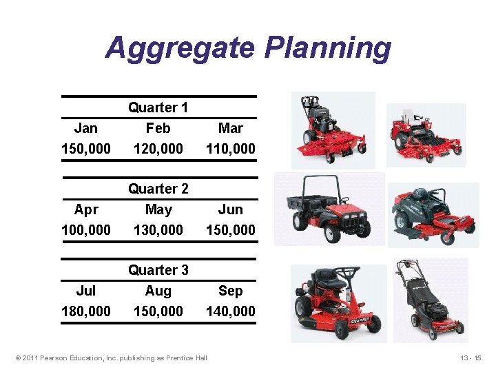
Lawn Mowers (aggregate unit) © 2011 Pearson Education, Inc. publishing as Prentice Hall 13 - 14

Aggregate Planning Jan 150, 000 Quarter 1 Feb 120, 000 Mar 110, 000 Apr 100, 000 Quarter 2 May 130, 000 Jun 150, 000 Jul 180, 000 Quarter 3 Aug 150, 000 Sep 140, 000 © 2011 Pearson Education, Inc. publishing as Prentice Hall 13 - 15

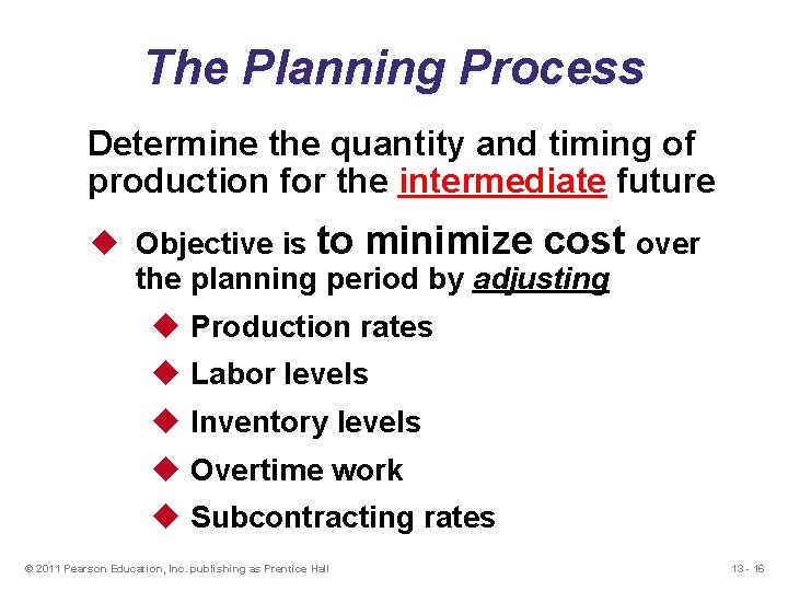
The Planning Process Determine the quantity and timing of production for the intermediate future u Objective is to minimize cost over the planning period by adjusting u Production rates u Labor levels u Inventory levels u Overtime work u Subcontracting rates © 2011 Pearson Education, Inc. publishing as Prentice Hall 13 - 16

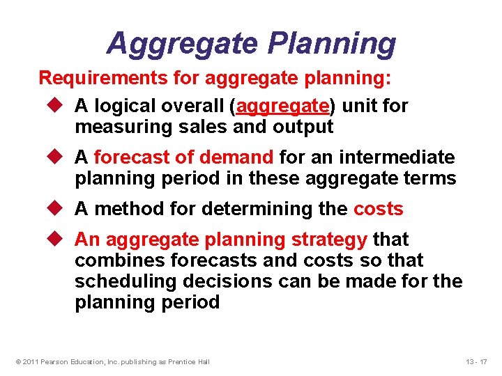
Aggregate Planning Requirements for aggregate planning: u A logical overall (aggregate) unit for measuring sales and output u A forecast of demand for an intermediate planning period in these aggregate terms u A method for determining the costs u An aggregate planning strategy that combines forecasts and costs so that scheduling decisions can be made for the planning period © 2011 Pearson Education, Inc. publishing as Prentice Hall 13 - 17

Aggregate Planning Strategies 1. Level Production: Maintaining a steady rate of production while meeting variations in demand by a combination of options ü Using part-timers, overtime, or idle time to absorb changes ü Using subcontractors and maintain a stable workforce ü Backordering, satisfying the demand of one period in one or more periods later. 2. Chase Demand: Matching capacity to demand by keeping production in each period equal to the expected demand for that period. 3. Mixed Strategies © 2011 Pearson Education, Inc. publishing as Prentice Hall 13 - 18

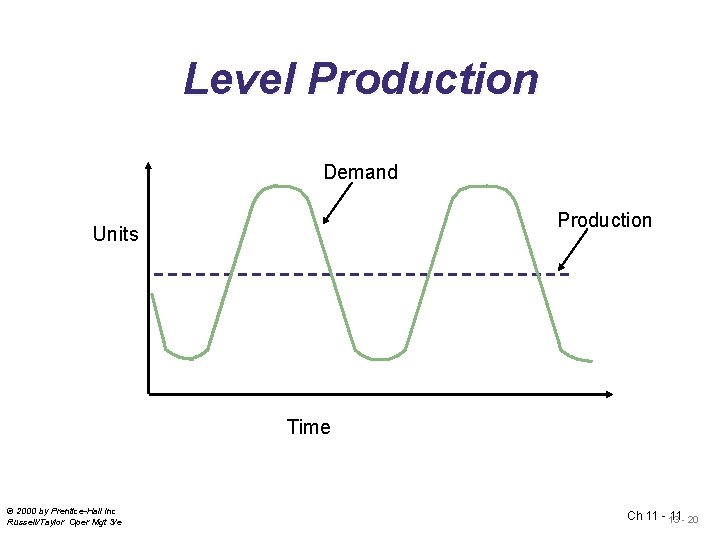
Level Production (Constant Workforce) u Daily production is uniform u Use inventory as buffer u The underlying philosophy is that stable employment leads to better quality, less turnover, less absenteeism, and more employee commitment. u This strategy works well when demand is stable © 2011 Pearson Education, Inc. publishing as Prentice Hall 13 - 19

Level Production Demand Production Units Time © 2000 by Prentice-Hall Inc Russell/Taylor Oper Mgt 3/e Ch 11 - 13 11 - 20

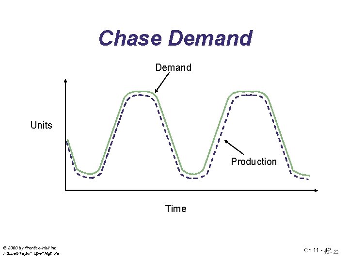
Chase Demand - Match output rates to demand forecast for each period by changing workforce levels or production rate - The disadvantages: a ready supply of skilled labor may not always available, newly hired personnel must be trained, and layoffs negatively affect the morale of all employees and maylead to a decrease in overall productivity. - Favored by many service organizations © 2011 Pearson Education, Inc. publishing as Prentice Hall 13 - 21

Chase Demand Units Production Time © 2000 by Prentice-Hall Inc Russell/Taylor Oper Mgt 3/e Ch 11 - 13 12 - 22

Mixed Strategies u Two or more options, such as overtime, subcontracting, hiring and layoff, etc. , are used. u There are both inventory changes and work force and production rate changes over the planning horizon. u Typically, mixed strategies are better (result in lower costs) than pure strategies © 2011 Pearson Education, Inc. publishing as Prentice Hall 13 - 23

Demand Capacity Options to Satisfy the Demand Over the Planning period u Proactive: Involve demand options: Attempt to change demand to match capacity ü Influence the demand ü Backordering ü Producing counter-seasonal products u Reactive: Involve capacity options: Attempt to change capacity to match demand ü Changing inventory Levels ü Varying workforce size by hiring or firing (layoffs) ü Varying production rate through overtime or idle time ü Subcontracting ü Using part-time workers 13 - 24

Capacity Options (Reactive) 1. Changing inventory levels u Increase inventory in low demand periods to meet high demand in the future u High inventory may increase costs associated with storage, insurance, handling, obsolescence, and capital investment u Low inventory may cause shortages which may mean lost sales due to long lead times and poor customer service © 2011 Pearson Education, Inc. publishing as Prentice Hall 13 - 25

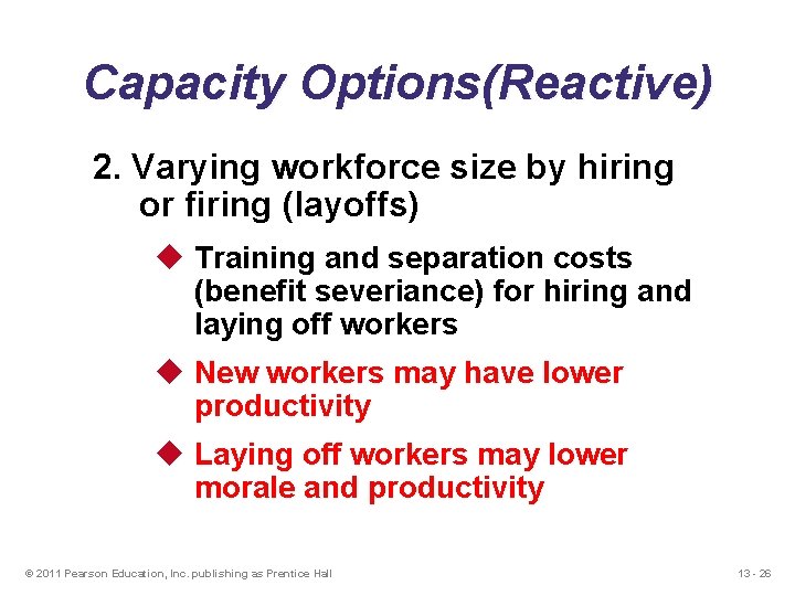
Capacity Options(Reactive) 2. Varying workforce size by hiring or firing (layoffs) u Training and separation costs (benefit severiance) for hiring and laying off workers u New workers may have lower productivity u Laying off workers may lower morale and productivity © 2011 Pearson Education, Inc. publishing as Prentice Hall 13 - 26

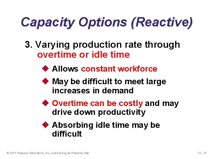
Capacity Options (Reactive) 3. Varying production rate through overtime or idle time u Allows constant workforce u May be difficult to meet large increases in demand u Overtime can be costly and may drive down productivity u Absorbing idle time may be difficult © 2011 Pearson Education, Inc. publishing as Prentice Hall 13 - 27

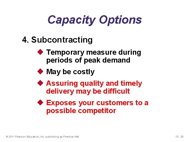
Capacity Options 4. Subcontracting u Temporary measure during periods of peak demand u May be costly u Assuring quality and timely delivery may be difficult u Exposes your customers to a possible competitor © 2011 Pearson Education, Inc. publishing as Prentice Hall 13 - 28

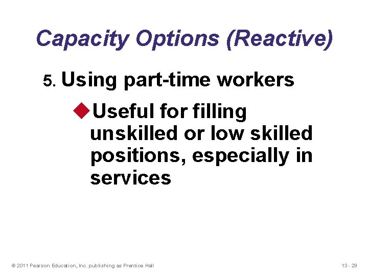
Capacity Options (Reactive) 5. Using part-time workers u. Useful for filling unskilled or low skilled positions, especially in services © 2011 Pearson Education, Inc. publishing as Prentice Hall 13 - 29

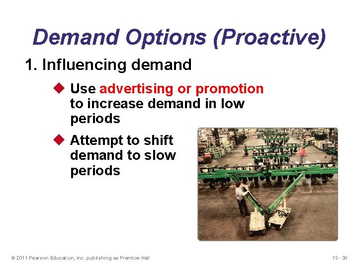
Demand Options (Proactive) 1. Influencing demand u Use advertising or promotion to increase demand in low periods u Attempt to shift demand to slow periods © 2011 Pearson Education, Inc. publishing as Prentice Hall 13 - 30

Demand Options 2. Back ordering during highdemand periods u Requires customers to wait for an order without loss of goodwill or the order u Most effective when there are few if any substitutes for the product or service u Often results in lost sales © 2011 Pearson Education, Inc. publishing as Prentice Hall 13 - 31

Demand Options 3. Producing counterseasonal products u Develop a product mix of counterseasonal items (furnaces and air conditioners) u However, may lead to products or services outside the company’s areas of expertise © 2011 Pearson Education, Inc. publishing as Prentice Hall 13 - 32

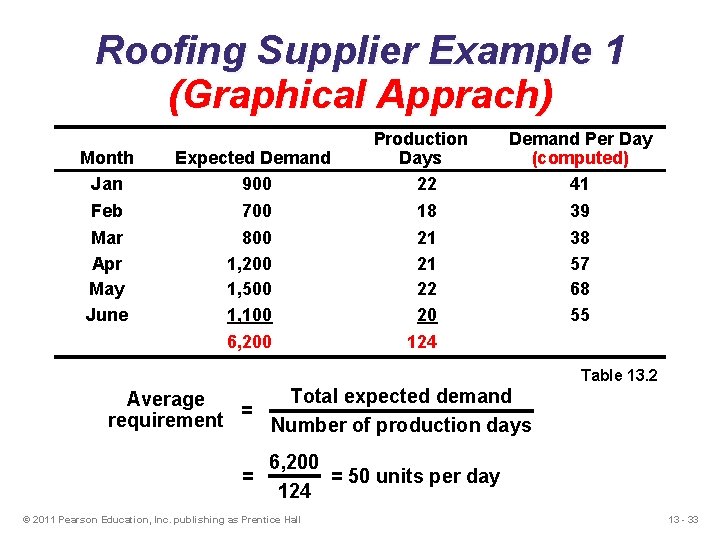
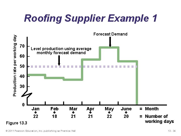
Roofing Supplier Example 1 (Graphical Apprach) Production Days 22 Month Jan Expected Demand 900 Feb Mar Apr May June 700 800 1, 200 1, 500 1, 100 18 21 21 22 20 6, 200 124 Demand Per Day (computed) 41 39 38 57 68 55 Table 13. 2 Total expected demand Average requirement = Number of production days = 6, 200 = 50 units per day 124 © 2011 Pearson Education, Inc. publishing as Prentice Hall 13 - 33

Production rate per working day Roofing Supplier Example 1 Forecast Demand 70 – 60 – Level production using average monthly forecast demand 50 – 40 – 30 – Jan Feb Mar Apr May June 22 18 21 21 22 20 Figure 13. 3 © 2011 Pearson Education, Inc. publishing as Prentice Hall = Month = Number of working days 13 - 34

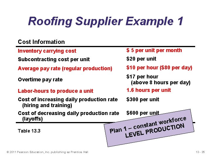
Roofing Supplier Example 1 Cost Information Inventory carrying cost $ 5 per unit per month Subcontracting cost per unit $20 per unit Average pay rate (regular production) $10 per hour ($80 per day) $17 per hour (above 8 hours per day) 1. 6 hours per unit Overtime pay rate Labor-hours to produce a unit Cost of increasing daily production rate (hiring and training) Cost of decreasing daily production rate (layoffs) Table 13. 3 © 2011 Pearson Education, Inc. publishing as Prentice Hall $300 per unit $600 per unit rce o f k r o nt w a t s n o ION c T – C 1 U n D Pla PRO L E V LE 13 - 35

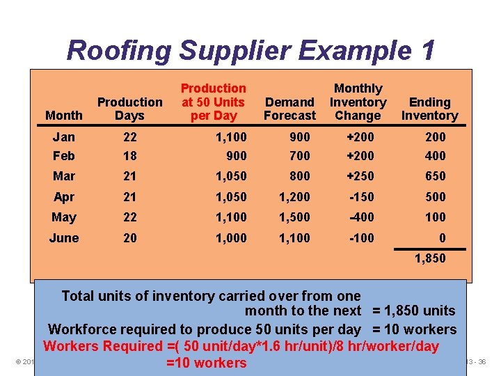
Roofing Supplier Example 1 Production Cost Information Production at 50 Units Month Days cost per Day Inventory carrying Jan 22 cost per unit 1, 100 Subcontracting Feb 18 900 Average pay rate Mar 21 1, 050 Overtime pay rate Apr 21 1, 050 Labor-hours to May 22 produce a unit 1, 100 Monthly Demand Inventory Ending Forecast Inventory $ 5 per. Change unit per month 900 200 $20 per +200 unit 700 $10 per +200 hour ($80 per 400 day) 800 +250 650 $17 per hour 8 hours per 500 day) 1, 200 (above-150 1. 6 hours per unit 1, 500 -400 100 $300 per-100 unit Cost Juneof increasing 20 daily production 1, 000 rate 1, 100 (hiring and training) Cost of decreasing daily production rate $600 per unit (layoffs) 0 1, 850 Total units of inventory carried over from one t workforce tan = 1, 850 units s n o Table 13. 3 monthnto the next c – Pla 1 Workforce required to produce 50 units per day = 10 workers Workers Required =( 50 unit/day*1. 6 hr/unit)/8 hr/worker/day © 2011 Pearson Education, Inc. publishing as Prentice Hall =10 workers 13 - 36

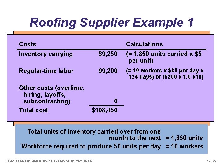
Roofing Supplier Example 1 Production Monthly Costs Calculations Cost Information Production Demand Ending at 50 Units Inventory Month Days cost per Day Inventory $ 5 per. Change unit per month Inventory carrying $9, 250 Forecast (= 1, 850 units carried x $5 per unit) Jan 22 cost per unit 1, 100 900 200 $20 per +200 unit Subcontracting Feb 18 labor 900 400 (=700 10 x $80 x Regular-time 99, 200 $10 workers per +200 hour ($80 per perday day) Average pay rate 124 or (6200 x 1. 6650 x 10) Mar 21 1, 050 800 days)+250 $17 per hour Overtime pay rate 8 hours per 500 day) Apr costs 21 1, 050 1, 200 (above-150 Other (overtime, hiring, layoffs, 1. 6 hours per unit Labor-hours to May 22 produce a unit 1, 100 1, 500 -400 100 subcontracting) 0 $300 per-100 unit Cost Juneof increasing 20 daily production 1, 000 rate 1, 100 Total cost $108, 450 (hiring and training) Cost of decreasing daily production rate $600 per unit (layoffs) 0 1, 850 Total units of inventory carried over from one t workforce tan = 1, 850 units s n o Table 13. 3 monthnto the next c – Pla 1 Workforce required to produce 50 units per day = 10 workers © 2011 Pearson Education, Inc. publishing as Prentice Hall 13 - 37

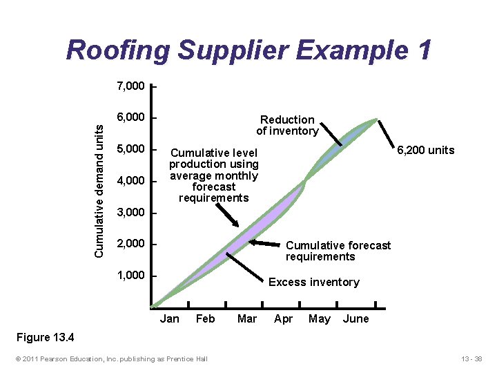
Roofing Supplier Example 1 7, 000 – Cumulative demand units 6, 000 – 5, 000 – 4, 000 – Reduction of inventory 6, 200 units Cumulative level production using average monthly forecast requirements 3, 000 – 2, 000 – Cumulative forecast requirements 1, 000 – – Excess inventory Jan Feb Mar Apr May June Figure 13. 4 © 2011 Pearson Education, Inc. publishing as Prentice Hall 13 - 38

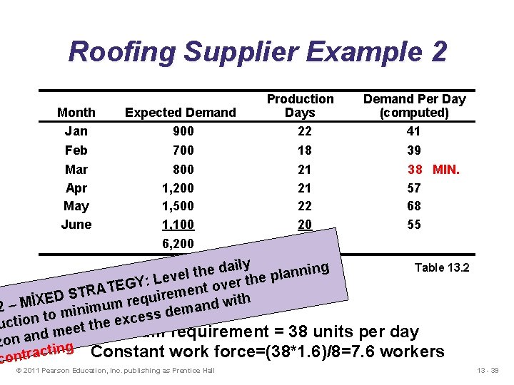
Roofing Supplier Example 2 Production Days 22 Month Jan Expected Demand 900 Feb Mar Apr May June 700 800 1, 200 1, 500 1, 100 18 21 21 22 20 6, 200 124 Demand Per Day (computed) 41 39 38 MIN. 57 68 55 Table 13. 2 daily ing e n h t n l a l e p v : Le r the Y e G v E o T t TRA men S e r i D u E q ith X re w d m n u 2 – Mİ a m dem mini s o s t e c n x o ucti he e t t e e Minimum requirement = 38 units per day dm zon an ng cti Constant work force=(38*1. 6)/8=7. 6 workers contra © 2011 Pearson Education, Inc. publishing as Prentice Hall 13 - 39

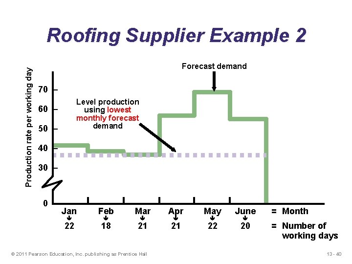
Production rate per working day Roofing Supplier Example 2 Forecast demand 70 – Level production using lowest monthly forecast demand 60 – 50 – 40 – 30 – Jan Feb Mar Apr May June 22 18 21 21 22 20 © 2011 Pearson Education, Inc. publishing as Prentice Hall = Month = Number of working days 13 - 40

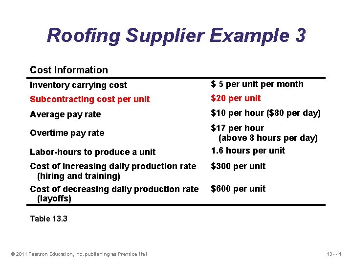
Roofing Supplier Example 3 Cost Information Inventory carrying cost $ 5 per unit per month Subcontracting cost per unit $20 per unit Average pay rate $10 per hour ($80 per day) Overtime pay rate Labor-hours to produce a unit Cost of increasing daily production rate (hiring and training) Cost of decreasing daily production rate (layoffs) $17 per hour (above 8 hours per day) 1. 6 hours per unit $300 per unit $600 per unit Table 13. 3 © 2011 Pearson Education, Inc. publishing as Prentice Hall 13 - 41

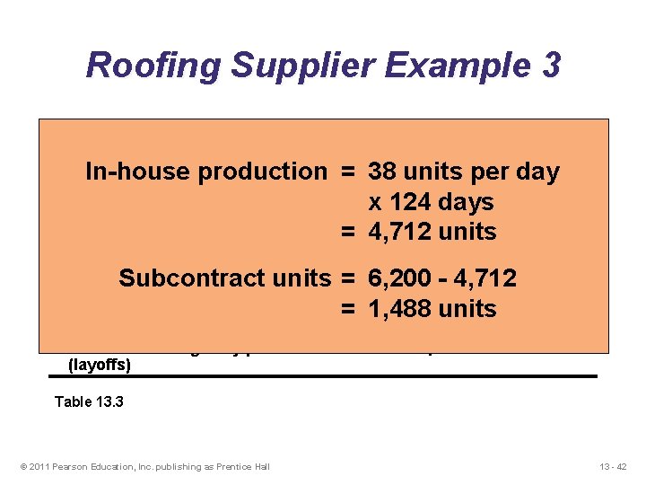
Roofing Supplier Example 3 Cost Information Inventory carry cost $ 5 per unit per month In-house production = 38$10 units per day per unit x $124 5 perdays hour ($40 per day) Average pay rate = 4, 712 $ 7 perunits hour Overtime pay rate Subcontracting cost per unit Labor-hours to produce a unit Subcontract units (above 8 hours per day) 1. 6 hours per unit 6, 200 - 4, 712 = $300 per unit Cost of increasing daily production rate = 1, 488 units (hiring and training) Cost of decreasing daily production rate (layoffs) $600 per unit Table 13. 3 © 2011 Pearson Education, Inc. publishing as Prentice Hall 13 - 42

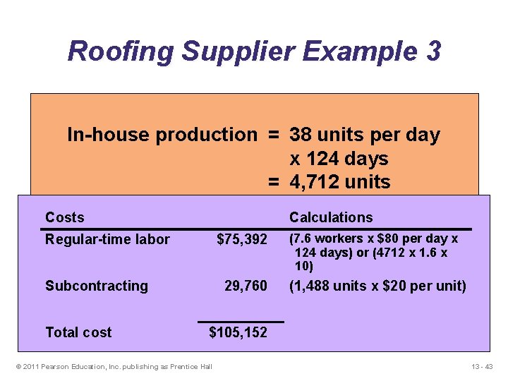
Roofing Supplier Example 3 Cost Information $ 5 per unit per month Inventory carry cost In-house production = 38$10 units per day per unit x $124 5 perdays hour ($40 per day) Average pay rate = 4, 712 $ 7 perunits hour Overtime pay rate Subcontracting cost per unit Costs Subcontract Labor-hours to produce a units (above 8 hours per day) 1. 6 hours per unit Calculations 6, 200 - 4, 712 = (7. 6 workers x $80 per day x Regular-time labor $75, 392 $300 per unit Cost of increasing daily production rate = 1, 488 units 124 days) or (4712 x 1. 6 x (hiring and training) 10) Cost of decreasing daily production rate $600 per unit Subcontracting 29, 760 (1, 488 units x $20 per unit) (layoffs) Table 13. 3 Total cost $105, 152 © 2011 Pearson Education, Inc. publishing as Prentice Hall 13 - 43

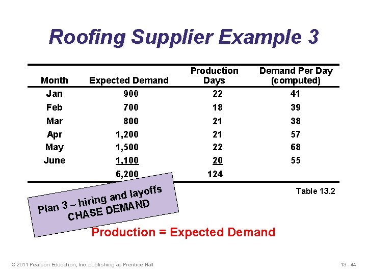
Roofing Supplier Example 3 Production Days 22 Month Jan Expected Demand 900 Feb Mar Apr May June 700 800 1, 200 1, 500 1, 100 18 21 21 22 20 6, 200 124 Demand Per Day (computed) 41 offs y a l d g an n i r i h D – Plan 3 ASE DEMAN CH 39 38 57 68 55 Table 13. 2 Production = Expected Demand © 2011 Pearson Education, Inc. publishing as Prentice Hall 13 - 44

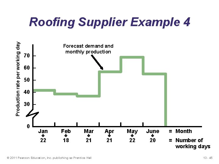
Production rate per working day Roofing Supplier Example 4 Forecast demand monthly production 70 – 60 – 50 – 40 – 30 – Jan Feb Mar Apr May June 22 18 21 21 22 20 © 2011 Pearson Education, Inc. publishing as Prentice Hall = Month = Number of working days 13 - 45

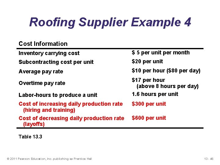
Roofing Supplier Example 4 Cost Information Inventory carrying cost $ 5 per unit per month Subcontracting cost per unit $20 per unit Average pay rate $10 per hour ($80 per day) Overtime pay rate Labor-hours to produce a unit Cost of increasing daily production rate (hiring and training) Cost of decreasing daily production rate (layoffs) $17 per hour (above 8 hours per day) 1. 6 hours per unit $300 per unit $600 per unit Table 13. 3 © 2011 Pearson Education, Inc. publishing as Prentice Hall 13 - 46

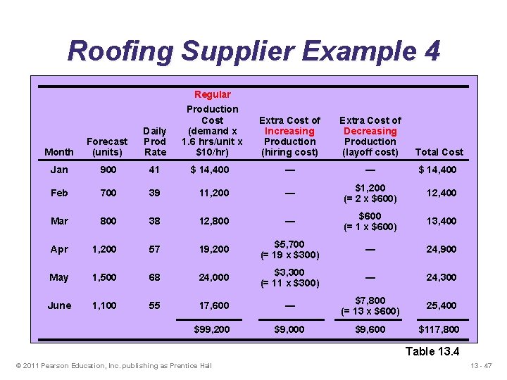
Roofing Supplier Example 4 Cost Information Regular Production Inventory carrying cost Cost (demand x Daily Prod per 1. 6 unit hrs/unit x Forecast cost Subcontracting Month Rate $10/hr) (units) Average pay Jan 900 rate Extra Cost$of 5 per. Extra unit. Cost perofmonth Increasing Decreasing Production $10 per. Production unit (hiring cost) (layoff cost) Total Cost 41 $ 14, 400 — Overtime pay rate 39 Feb 700 11, 200 — Labor-hours a 12, 800 unit Mar 800 to produce 38 — $ 5 per hour ($40 per day) — $ 14, 400 $ 7 per hour $1, 200 12, 400 (= 28 x hours $600) per day) (above 1. 6 hours$600 per unit 13, 400 (= 1 x $600) Cost of increasing daily production rate $5, 700$300 per unit Apr 1, 200 57 19, 200 — (hiring and training) (= 19 x $300) $3, 300$600 per unit Cost rate May of decreasing 1, 500 68 daily production 24, 000 — (= 11 x $300) (layoffs) June 1, 100 Table 13. 3 55 24, 900 24, 300 17, 600 — $7, 800 (= 13 x $600) 25, 400 $99, 200 $9, 000 $9, 600 $117, 800 Table 13. 4 © 2011 Pearson Education, Inc. publishing as Prentice Hall 13 - 47

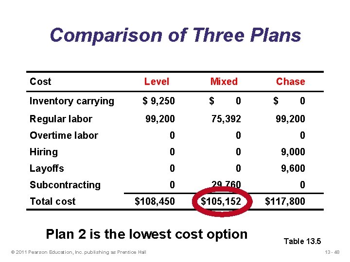
Comparison of Three Plans Cost Level Mixed Inventory carrying $ 9, 250 $ Regular labor 99, 200 75, 392 99, 200 Overtime labor 0 0 0 Hiring 0 0 9, 000 Layoffs 0 0 9, 600 Subcontracting 0 29, 760 0 $108, 450 $105, 152 $117, 800 Total cost 0 Plan 2 is the lowest cost option © 2011 Pearson Education, Inc. publishing as Prentice Hall Chase $ 0 Table 13. 5 13 - 48

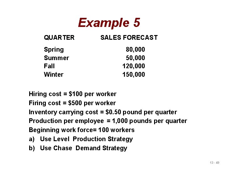
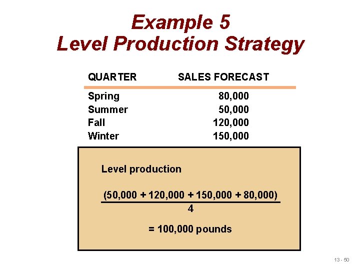
Example 5 QUARTER Spring Summer Fall Winter SALES FORECAST 80, 000 50, 000 120, 000 150, 000 Hiring cost = $100 per worker Firing cost = $500 per worker Inventory carrying cost = $0. 50 pound per quarter Production per employee = 1, 000 pounds per quarter Beginning work force= 100 workers a) Use Level Production Strategy b) Use Chase Demand Strategy 13 - 49

Example 5 Level Production Strategy QUARTER SALES FORECAST Spring Summer Fall Winter 80, 000 50, 000 120, 000 150, 000 Level production (50, 000 + 120, 000 + 150, 000 + 80, 000) 4 = 100, 000 pounds 13 - 50

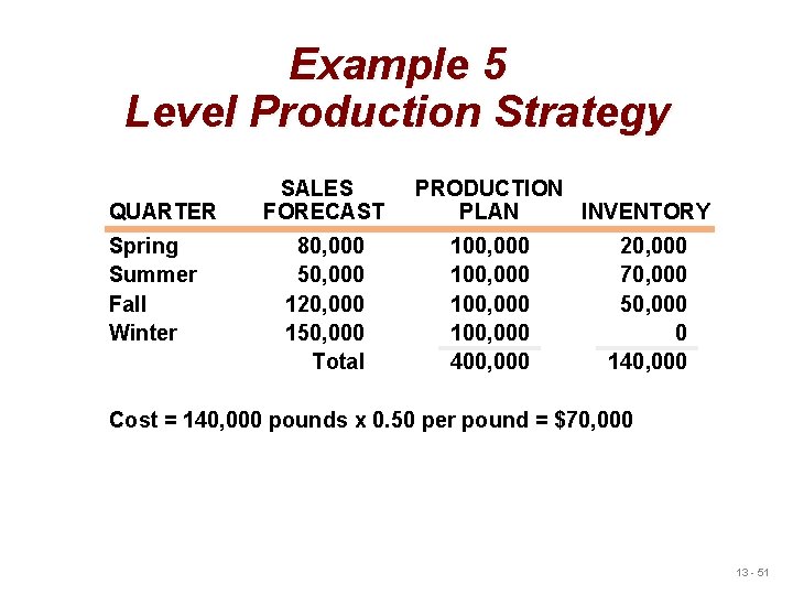
Example 5 Level Production Strategy QUARTER Spring Summer Fall Winter SALES FORECAST 80, 000 50, 000 120, 000 150, 000 Total PRODUCTION PLAN INVENTORY 100, 000 400, 000 20, 000 70, 000 50, 000 0 140, 000 Cost = 140, 000 pounds x 0. 50 per pound = $70, 000 13 - 51

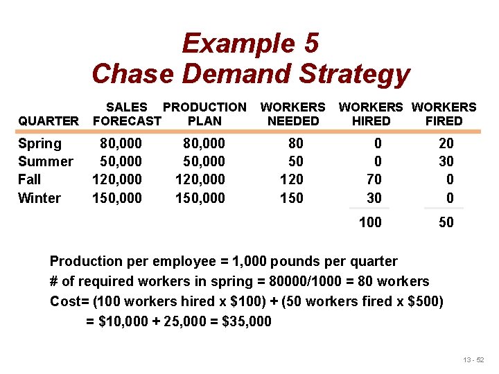
Example 5 Chase Demand Strategy QUARTER SALES PRODUCTION FORECAST PLAN Spring Summer Fall Winter 80, 000 50, 000 120, 000 150, 000 WORKERS NEEDED 80 50 120 150 WORKERS HIRED FIRED 0 0 70 30 20 30 0 0 100 50 Production per employee = 1, 000 pounds per quarter # of required workers in spring = 80000/1000 = 80 workers Cost= (100 workers hired x $100) + (50 workers fired x $500) = $10, 000 + 25, 000 = $35, 000 13 - 52

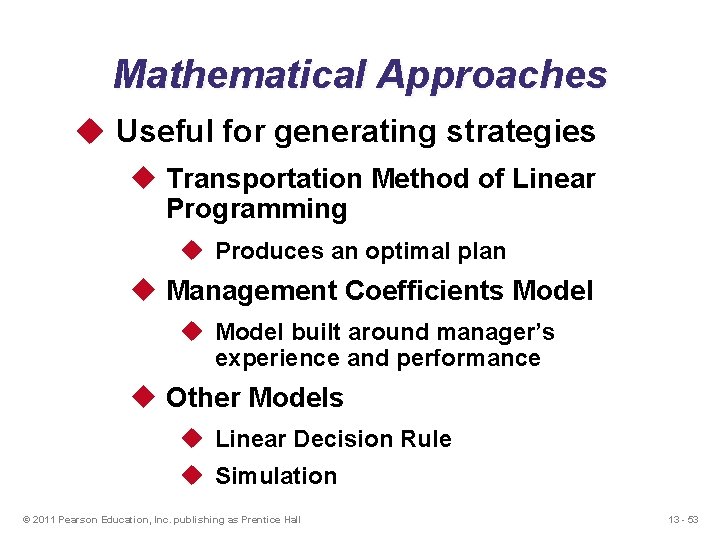
Mathematical Approaches u Useful for generating strategies u Transportation Method of Linear Programming u Produces an optimal plan u Management Coefficients Model u Model built around manager’s experience and performance u Other Models u Linear Decision Rule u Simulation © 2011 Pearson Education, Inc. publishing as Prentice Hall 13 - 53

Disaggregation of Aggregate Plan u Working with aggregate units facilitates intermediate planning. u But to put this plan into action we should decompose it, in other words, disaggregate it and state it in terms of actual units of products and plan the production for a shorter period of time u Breaking down aggregate product to real specific products helps to calculate manpower, material and inventory requirements in detail. u Disaggregation results in a Master Production Schedule (MPS) and MPS becomes input to Material Requirements Planning (MRP). © 2011 Pearson Education, Inc. publishing as Prentice Hall 13 - 54

Master Production Schedule u It indicates the quantity and timing of planned production by taking into account desired delivery quantity and timing as well as on-hand inventory. u The MPS is one of the primary outputs of the master scheduling process. 13 - 55

Rough-cut capacity Planning (RCCP) u RCCP involves testing the feasibility of a proposed MASTER SCHEDULE relative to available capacities, to assure that no obvious capacity constraints exist. © 2011 Pearson Education, Inc. publishing as Prentice Hall 13 - 56

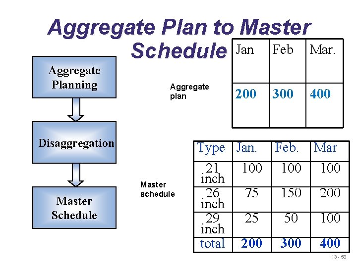
Disaggregating the aggregate plan u For example, televisions manufacturer may have an aggregate plan that calls for 200 television in January, 300 in February, and 400 in March. u This company produces 21, 26, and 29 inch TVs, therefore this three-month aggregate plan must be translated into specific numbers of TVs of each type (Master Schedule) prior to actually purchasing the appropriate materials and parts, scheduling operations, and planning inventory requirements. 13 - 57

Aggregate Plan to Master Schedule Jan Feb Mar. Aggregate Planning Aggregate plan Disaggregation Master Schedule Master schedule 200 300 400 Type Jan. Feb. Mar 21 100 100 inch 26 75 150 200 inch 29 25 50 100 inch total 200 300 400 13 - 58

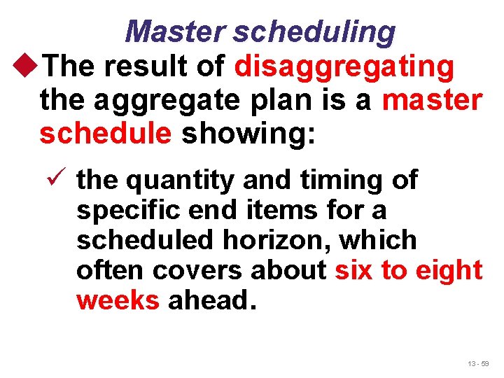
Master scheduling u. The result of disaggregating the aggregate plan is a master schedule showing: ü the quantity and timing of specific end items for a scheduled horizon, which often covers about six to eight weeks ahead. 13 - 59

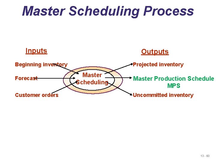
Master Scheduling Process Inputs Outputs Beginning inventory Forecast Customer orders Projected inventory Master Scheduling Master Production Schedule MPS Uncommitted inventory 13 - 60

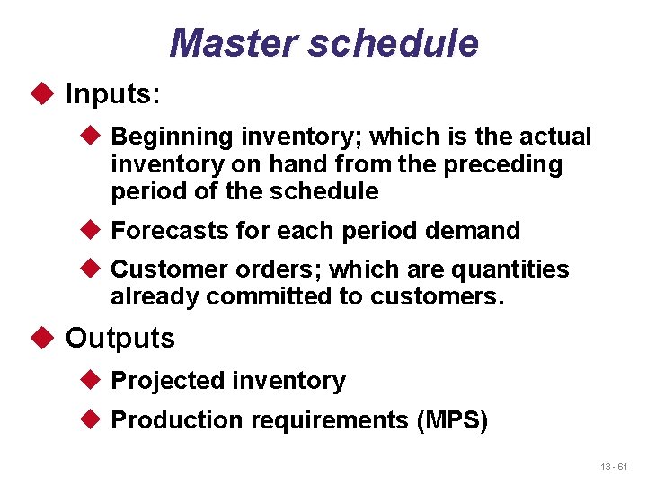
Master schedule u Inputs: u Beginning inventory; which is the actual inventory on hand from the preceding period of the schedule u Forecasts for each period demand u Customer orders; which are quantities already committed to customers. u Outputs u Projected inventory u Production requirements (MPS) 13 - 61

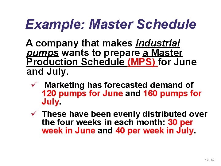
Example: Master Schedule A company that makes industrial pumps wants to prepare a Master Production Schedule (MPS) for June and July. ü Marketing has forecasted demand of 120 pumps for June and 160 pumps for July. ü These have been evenly distributed over the four weeks in each month: 30 per week in June and 40 per week in July. 13 - 62

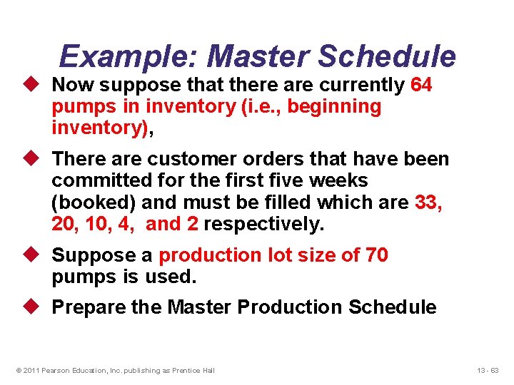
Example: Master Schedule u Now suppose that there are currently 64 pumps in inventory (i. e. , beginning inventory), u There are customer orders that have been committed for the first five weeks (booked) and must be filled which are 33, 20, 10, 4, and 2 respectively. u Suppose a production lot size of 70 pumps is used. u Prepare the Master Production Schedule © 2011 Pearson Education, Inc. publishing as Prentice Hall 13 - 63

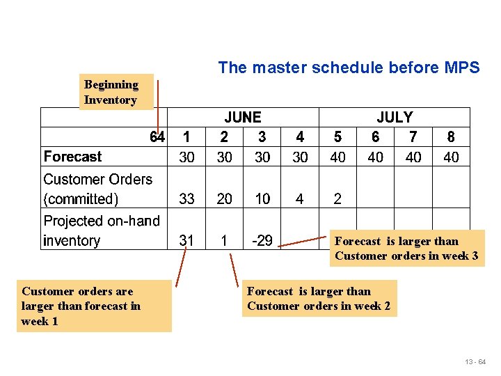
The master schedule before MPS Beginning Inventory Forecast is larger than Customer orders in week 3 Customer orders are larger than forecast in week 1 Forecast is larger than Customer orders in week 2 13 - 64

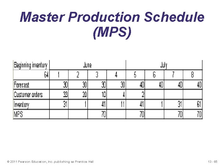
Master Production Schedule (MPS) © 2011 Pearson Education, Inc. publishing as Prentice Hall 13 - 65

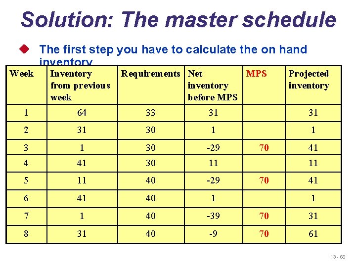
Solution: The master schedule u The first step you have to calculate the on hand inventory Week Inventory from previous week Requirements Net MPS inventory before MPS Projected inventory 1 64 33 31 31 2 31 30 1 1 30 -29 4 41 30 11 5 11 40 -29 6 41 40 1 7 1 40 -39 70 31 8 31 40 -9 70 61 70 41 1 13 - 66

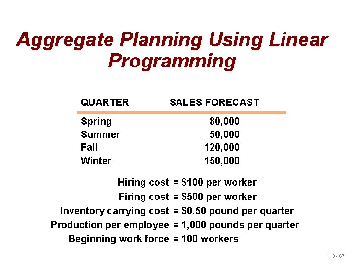
Aggregate Planning Using Linear Programming QUARTER Spring Summer Fall Winter Hiring cost Firing cost Inventory carrying cost Production per employee Beginning work force SALES FORECAST 80, 000 50, 000 120, 000 150, 000 = $100 per worker = $500 per worker = $0. 50 pound per quarter = 1, 000 pounds per quarter = 100 workers 13 - 67

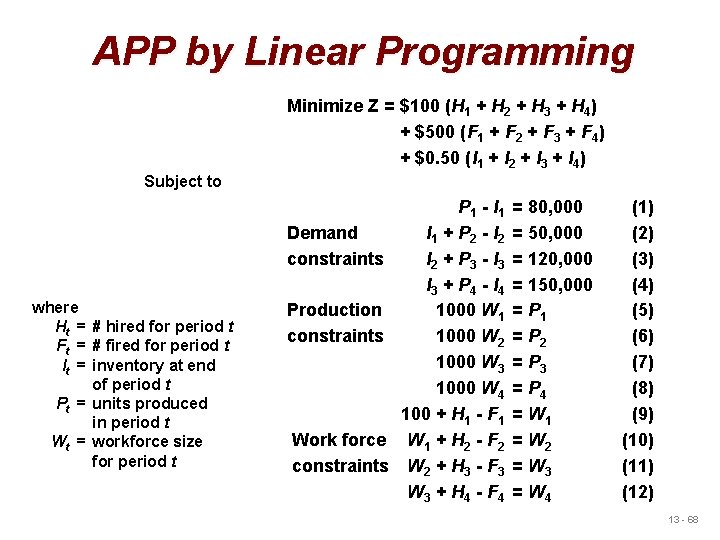
APP by Linear Programming Minimize Z = $100 (H 1 + H 2 + H 3 + H 4) + $500 (F 1 + F 2 + F 3 + F 4) + $0. 50 (I 1 + I 2 + I 3 + I 4) Subject to Demand constraints where Ht = # hired for period t Ft = # fired for period t It = inventory at end of period t Pt = units produced in period t Wt = workforce size for period t Production constraints Work force constraints P 1 - I 1 + P 2 - I 2 + P 3 - I 3 + P 4 - I 4 1000 W 1 1000 W 2 1000 W 3 1000 W 4 100 + H 1 - F 1 W 1 + H 2 - F 2 W 2 + H 3 - F 3 W 3 + H 4 - F 4 = 80, 000 = 50, 000 = 120, 000 = 150, 000 = P 1 = P 2 = P 3 = P 4 = W 1 = W 2 = W 3 = W 4 (1) (2) (3) (4) (5) (6) (7) (8) (9) (10) (11) (12) 13 - 68

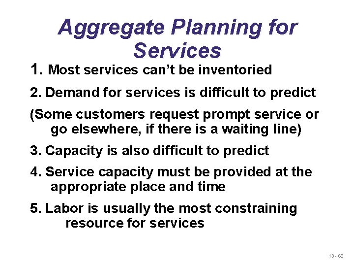
Aggregate Planning for Services 1. Most services can’t be inventoried 2. Demand for services is difficult to predict (Some customers request prompt service or go elsewhere, if there is a waiting line) 3. Capacity is also difficult to predict 4. Service capacity must be provided at the appropriate place and time 5. Labor is usually the most constraining resource for services 13 - 69

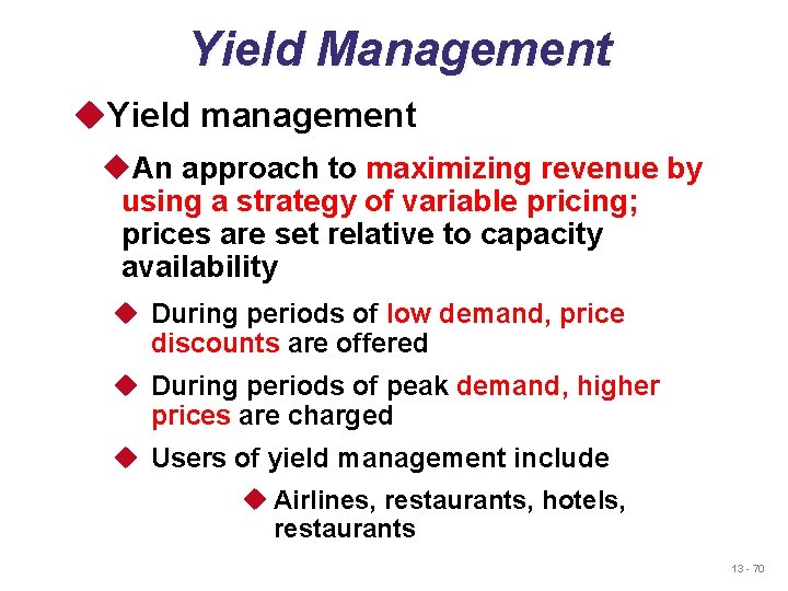
Yield Management u. Yield management u. An approach to maximizing revenue by using a strategy of variable pricing; prices are set relative to capacity availability u During periods of low demand, price discounts are offered u During periods of peak demand, higher prices are charged u Users of yield management include u Airlines, restaurants, hotels, restaurants 13 - 70

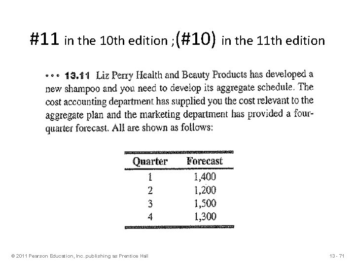
#11 in the 10 th edition ; (#10) in the 11 th edition © 2011 Pearson Education, Inc. publishing as Prentice Hall 13 - 71

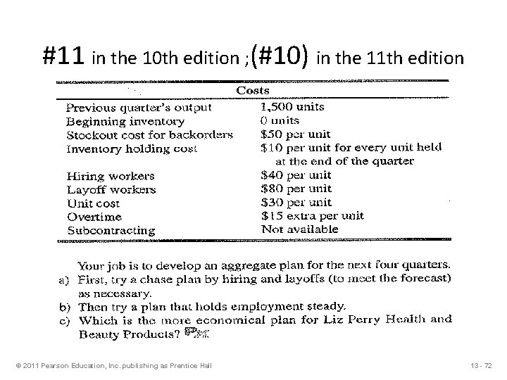
#11 in the 10 th edition ; (#10) in the 11 th edition © 2011 Pearson Education, Inc. publishing as Prentice Hall 13 - 72

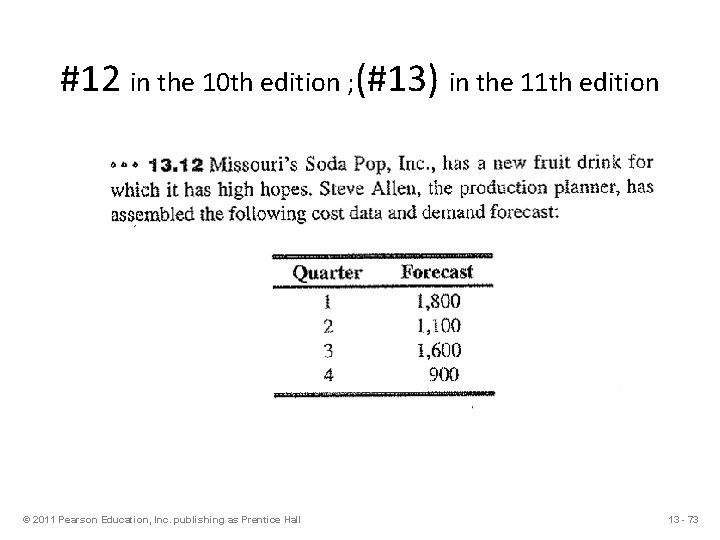
#12 in the 10 th edition ; (#13) in the 11 th edition © 2011 Pearson Education, Inc. publishing as Prentice Hall 13 - 73

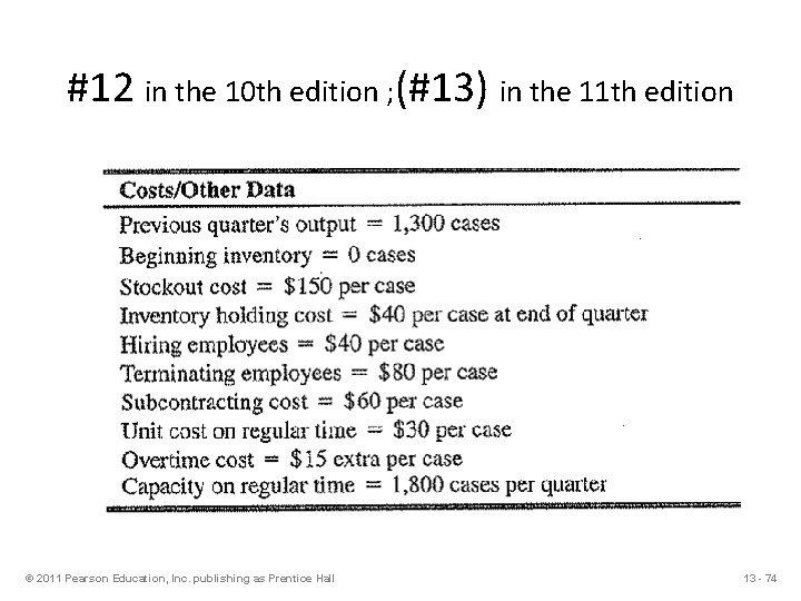
#12 in the 10 th edition ; (#13) in the 11 th edition © 2011 Pearson Education, Inc. publishing as Prentice Hall 13 - 74

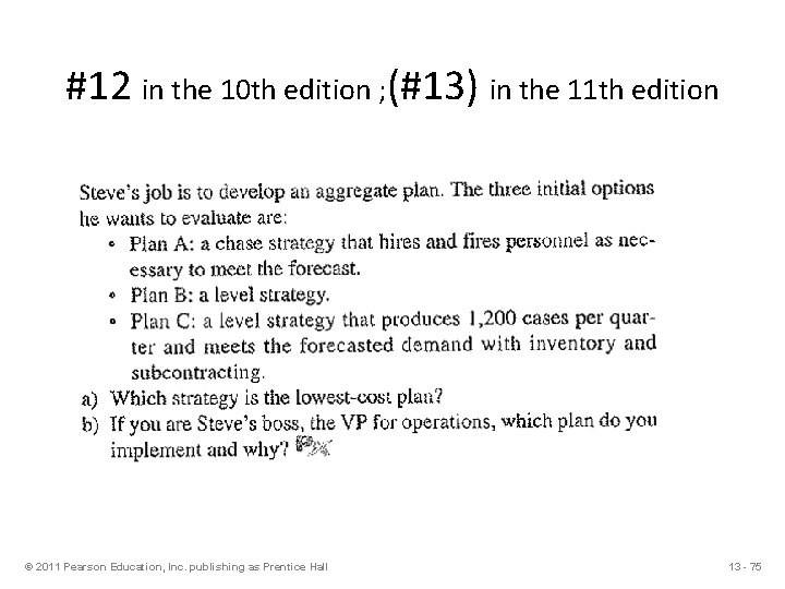
#12 in the 10 th edition ; (#13) in the 11 th edition © 2011 Pearson Education, Inc. publishing as Prentice Hall 13 - 75