Adaptive Query Processing with Eddies Amol Deshpande University

Adaptive Query Processing with Eddies Amol Deshpande University of Maryland

Roadmap n Adaptive Query Processing: Motivation n Eddies [AH’ 00] n STAIRs [DH’ 04] and Ste. Ms [RDH’ 03] n Experimental Study n Implementation in Postgre. SQL [Des’ 03] n Continuous queries [MSHR’ 02] (very briefly) n Open problems

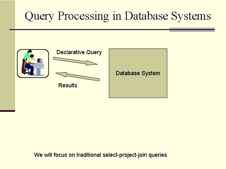
Query Processing in Database Systems Declarative Query Database System Results We will focus on traditional select-project-join queries

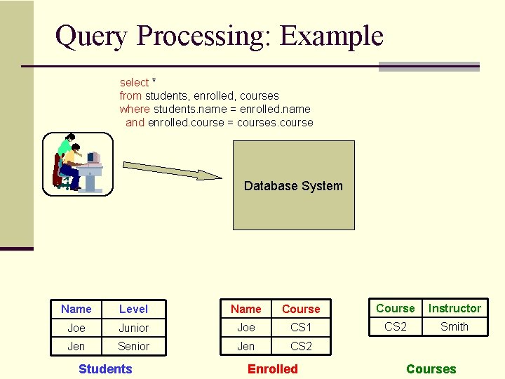
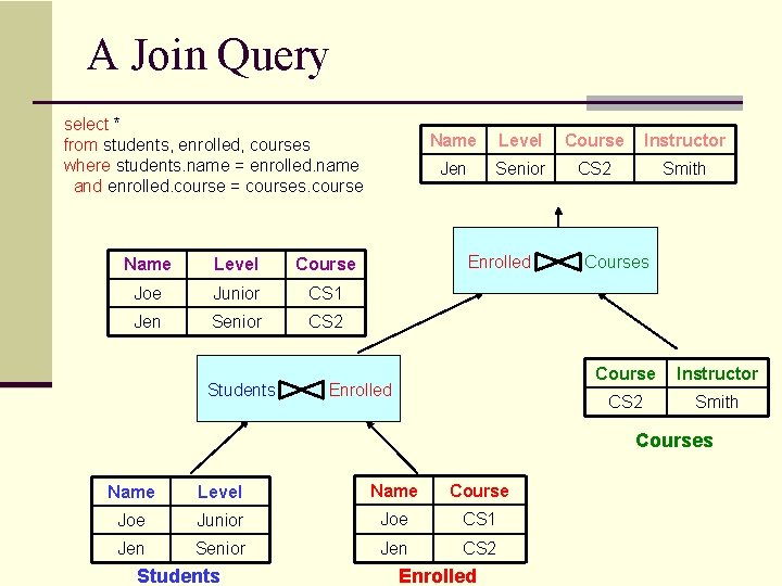
Query Processing: Example select * from students, enrolled, courses where students. name = enrolled. name and enrolled. course = courses. course Database System Name Level Name Course Instructor Joe Junior Joe CS 1 CS 2 Smith Jen Senior Jen CS 2 Students Enrolled Courses

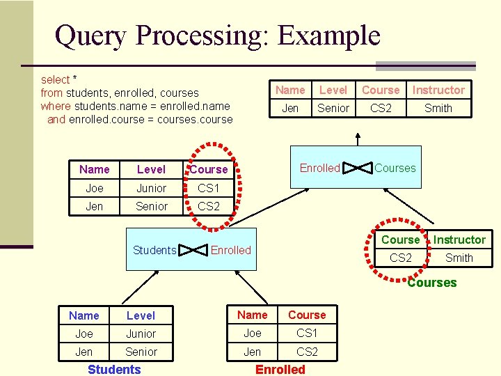
Query Processing: Example select * from students, enrolled, courses where students. name = enrolled. name and enrolled. course = courses. course Name Level Course Joe Junior CS 1 Jen Senior CS 2 Students Name Level Course Instructor Jen Senior CS 2 Smith Enrolled Courses Course Instructor CS 2 Smith Courses Name Level Name Course Joe Junior Joe CS 1 Jen Senior Jen CS 2 Students Enrolled

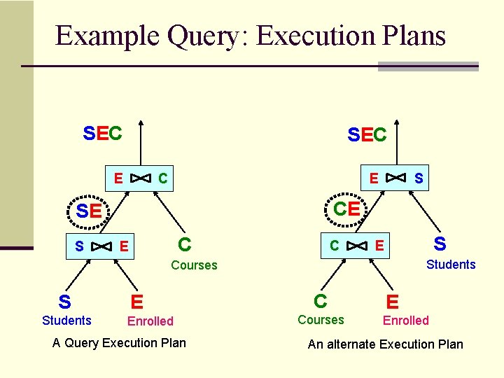
Example Query: Execution Plans SEC E E C CE SE S S C E C S E Students Courses S Students E Enrolled A Query Execution Plan C Courses E Enrolled An alternate Execution Plan

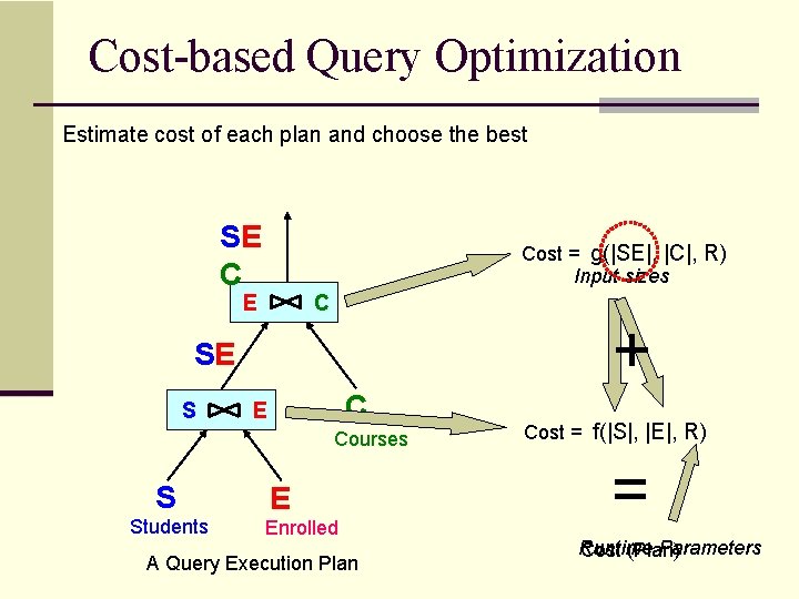
Cost-based Query Optimization Estimate cost of each plan and choose the best SE C Cost = g(|SE|, |C|, R) Input sizes E C + SE S C E Courses S Students E Enrolled A Query Execution Plan Cost = f(|S|, |E|, R) = Runtime Parameters Cost (Plan)

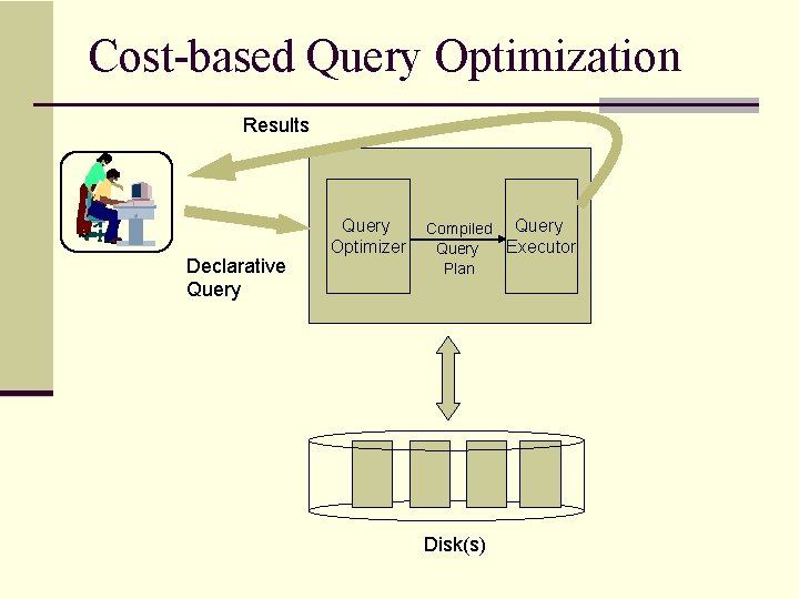
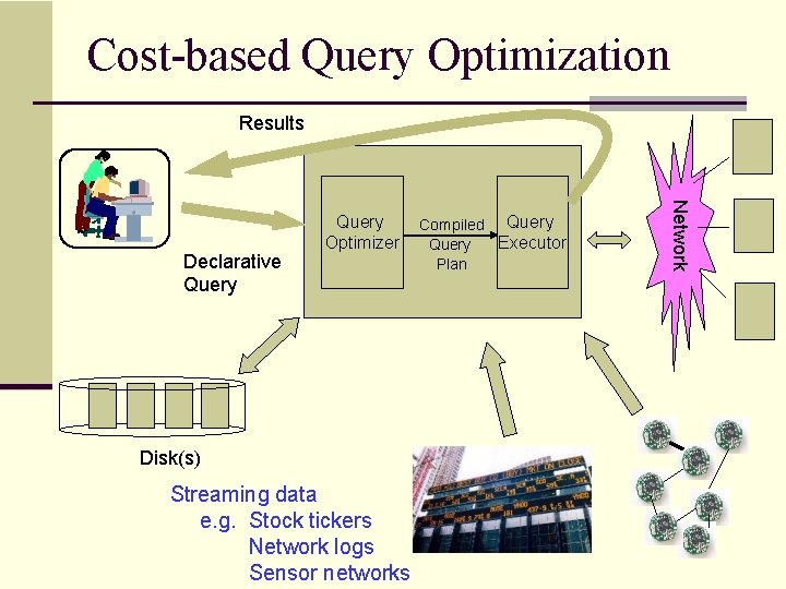
Cost-based Query Optimization Results Declarative Query Optimizer Compiled Query Executor Query Plan Disk(s)

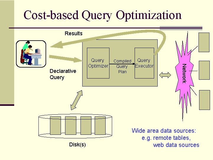
Cost-based Query Optimization Results Disk(s) Compiled Query Executor Query Plan Network Declarative Query Optimizer Wide area data sources: e. g. remote tables, web data sources

Cost-based Query Optimization Results Disk(s) Streaming data e. g. Stock tickers Network logs Sensor networks Compiled Query Executor Query Plan Network Declarative Query Optimizer

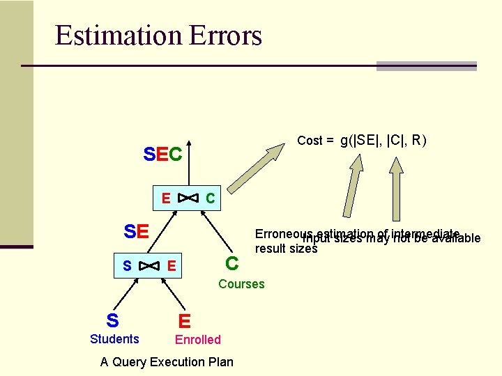
Estimation Errors Cost = g(|SE|, |C|, R) SEC E C SE S C E Erroneous estimation of intermediate Input sizes may not be available result sizes Courses S Students E Enrolled A Query Execution Plan

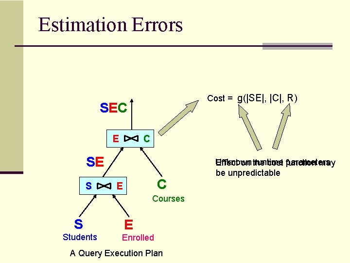
Estimation Errors Cost = g(|SE|, |C|, R) SEC E C SE S C E Courses S Students E Enrolled A Query Execution Plan Unknown runtime parameters Effect on the cost function may be unpredictable

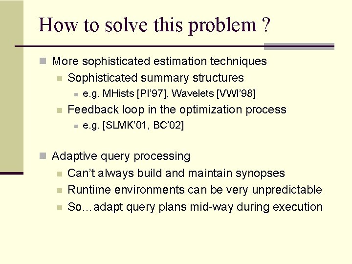
How to solve this problem ? n More sophisticated estimation techniques n Sophisticated summary structures n n e. g. MHists [PI’ 97], Wavelets [VWI’ 98] Feedback loop in the optimization process n e. g. [SLMK’ 01, BC’ 02] n Adaptive query processing n n n Can’t always build and maintain synopses Runtime environments can be very unpredictable So…adapt query plans mid-way during execution

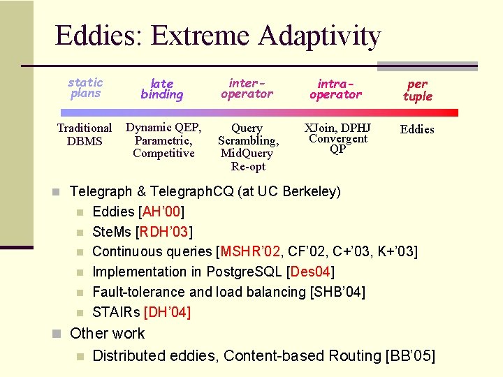
Eddies: Extreme Adaptivity static plans late binding interoperator intraoperator per tuple Traditional DBMS Dynamic QEP, Parametric, Competitive Query Scrambling, Mid. Query Re-opt XJoin, DPHJ Convergent QP Eddies n Telegraph & Telegraph. CQ (at UC Berkeley) n n n Eddies [AH’ 00] Ste. Ms [RDH’ 03] Continuous queries [MSHR’ 02, CF’ 02, C+’ 03, K+’ 03] Implementation in Postgre. SQL [Des 04] Fault-tolerance and load balancing [SHB’ 04] STAIRs [DH’ 04] n Other work n Distributed eddies, Content-based Routing [BB’ 05]

Roadmap n Adaptive Query Processing: Motivation n Eddies [AH’ 00] n STAIRs [DH’ 04] and Ste. Ms [RDH’ 03] n Experimental Study n Implementation in Postgre. SQL [Des’ 03] n Continuous queries [MSHR’ 02] (very briefly) n Open problems

Eddies [AH’ 00] select * from S where pred 1(S) and pred 2(S) Plans considered by the optimizer S pred 1(S) pred 2(S) Output S pred 2(S) pred 1(S) Output Decision made apriori based on statistics Sort by (1 -s)/c, where s = selectivity, c = cost Once this decision is made, all tuples are processed using the same order

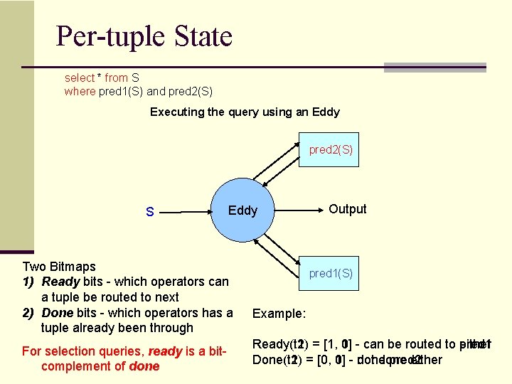
Eddies [AH’ 00] select * from S where pred 1(S) and pred 2(S) Executing the query using an Eddy pred 2(S) S An eddy operator • Intercepts tuples from source(s) and output tuples from operators • Query executed by routing tuples between the operators • Uses feedback from the operators to route Eddy Output pred 1(S) Change routing ==> Change query execution plan used

Per-tuple State select * from S where pred 1(S) and pred 2(S) Executing the query using an Eddy pred 2(S) S Eddy Two Bitmaps 1) Ready bits - which operators can a tuple be routed to next 2) Done bits - which operators has a tuple already been through For selection queries, ready is a bitcomplement of done Output pred 1(S) Example: Ready(t 2) = [1, 0] Ready(t 1) 1] - can be routed to either pred 1 Done(t 1) = [0, 1] Done(t 2) 0] - not done pred 2 either

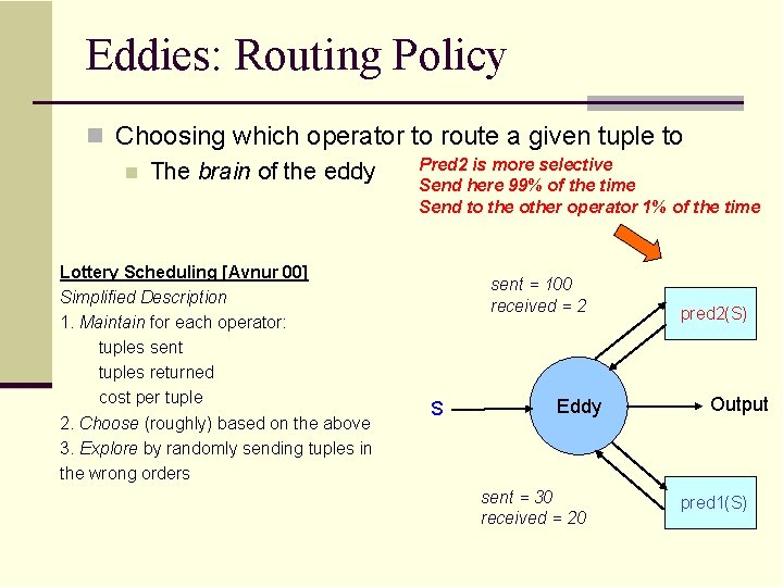
Eddies: Routing Policy n Choosing which operator to route a given tuple to Pred 2 is more selective n The brain of the eddy Send here 99% of the time Send to the other operator 1% of the time Lottery Scheduling [Avnur 00] Simplified Description 1. Maintain for each operator: tuples sent tuples returned cost per tuple 2. Choose (roughly) based on the above 3. Explore by randomly sending tuples in the wrong orders sent = 100 received = 2 S Eddy sent = 30 received = 20 pred 2(S) Output pred 1(S)

A Join Query select * from students, enrolled, courses where students. name = enrolled. name and enrolled. course = courses. course Name Level Course Joe Junior CS 1 Jen Senior CS 2 Students Name Level Course Instructor Jen Senior CS 2 Smith Enrolled Courses Course Instructor CS 2 Smith Courses Name Level Name Course Joe Junior Joe CS 1 Jen Senior Jen CS 2 Students Enrolled

Eddies [AH’ 00] Query execution using an eddy A traditional query plan Output E S S C C E S E C Output Eddy E S E A key difference: Tuples can’t be arbitrarily routed to any operator E. g. S tuples can’t be routed to E Join C Use ready bits to identify this E C

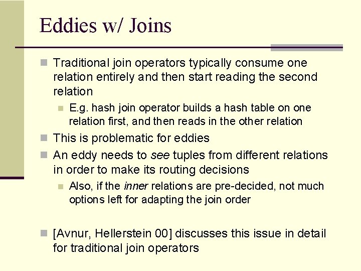
Eddies w/ Joins n Traditional join operators typically consume one relation entirely and then start reading the second relation n E. g. hash join operator builds a hash table on one relation first, and then reads in the other relation n This is problematic for eddies n An eddy needs to see tuples from different relations in order to make its routing decisions n Also, if the inner relations are pre-decided, not much options left for adapting the join order n [Avnur, Hellerstein 00] discusses this issue in detail for traditional join operators

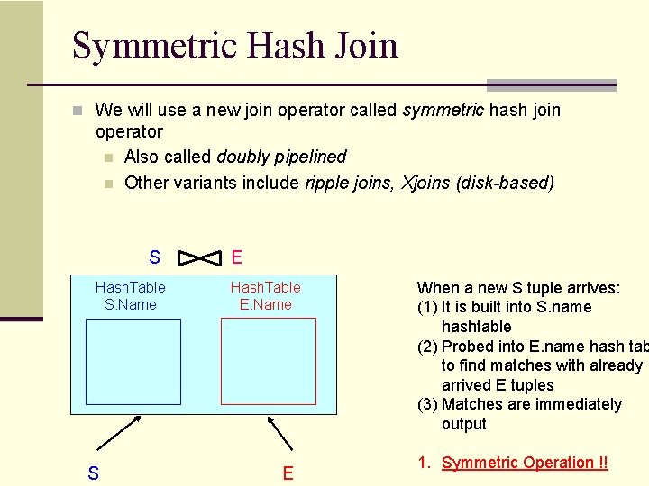
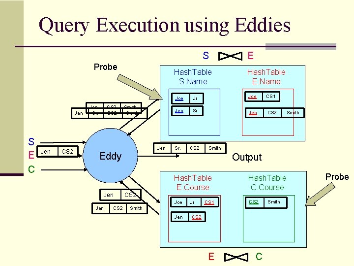
Symmetric Hash Join n We will use a new join operator called symmetric hash join operator n Also called doubly pipelined n Other variants include ripple joins, Xjoins (disk-based) S Hash. Table S. Name S E Hash. Table E. Name E When a new S tuple arrives: (1) It is built into S. name hashtable (2) Probed into E. name hash tab to find matches with already arrived E tuples (3) Matches are immediately output 1. Symmetric Operation !!

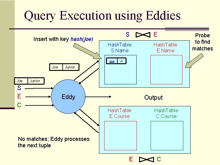
Query Execution using Eddies Insert with key hash(joe) S Hash. Table S. Name Joe Joe S E C E Hash. Table E. Name Jr Junior Eddy Output Hash. Table E. Course Hash. Table C. Course No matches; Eddy processes the next tuple E C Probe to find matches

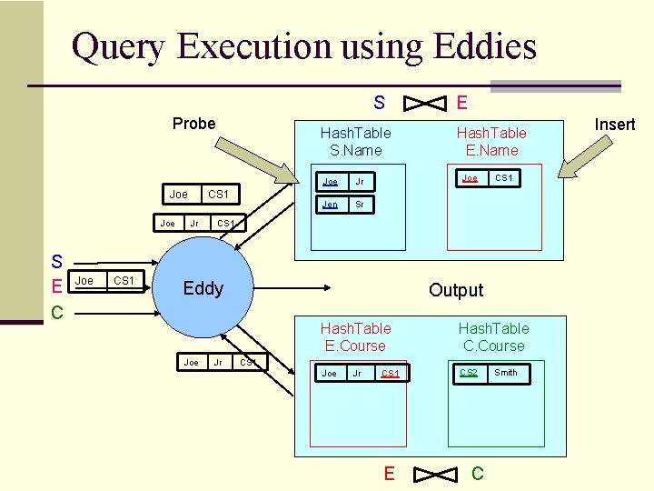
Query Execution using Eddies S Probe Joe S E C Joe CS 1 Hash. Table S. Name CS 1 Jr Joe Jr Jen Sr Hash. Table E. Name Joe CS 1 Eddy Joe E Jr Output Hash. Table E. Course Hash. Table C. Course Joe CS 2 CS 1 Jr CS 1 E C Smith Insert

Query Execution using Eddies S Probe Jen S E C Jen CS 2 Jen Sr. CS 2 Smith Jen Eddy Jen CS 2 E Hash. Table S. Name Hash. Table E. Name Joe Jr Joe CS 1 Jen Sr Jen CS 2 Sr. CS 2 Smith Output CS 2 Hash. Table E. Course Hash. Table C. Course Joe CS 2 Jr CS 1 Smith Jen CS 2 E C Smith Probe

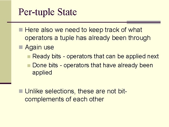
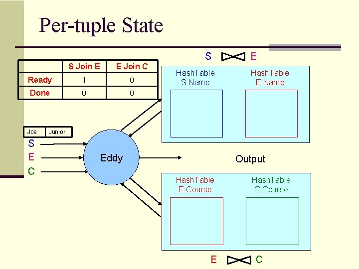
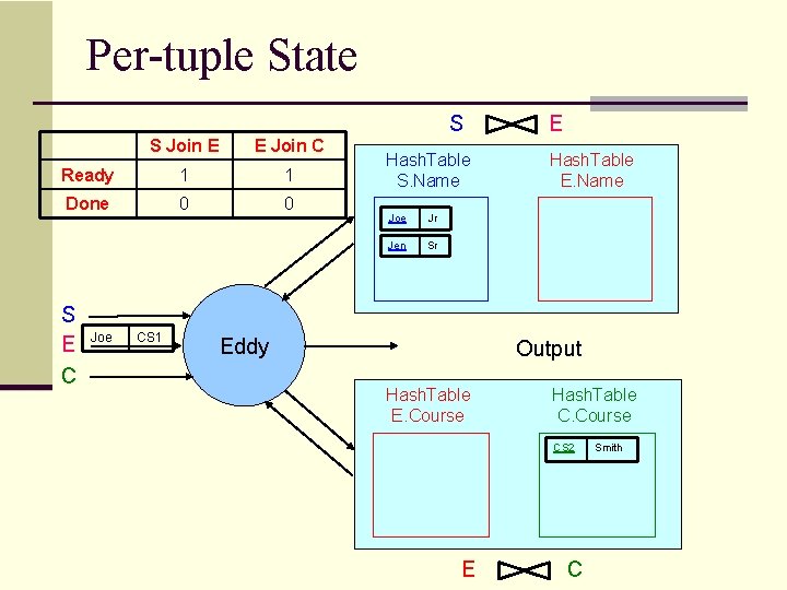
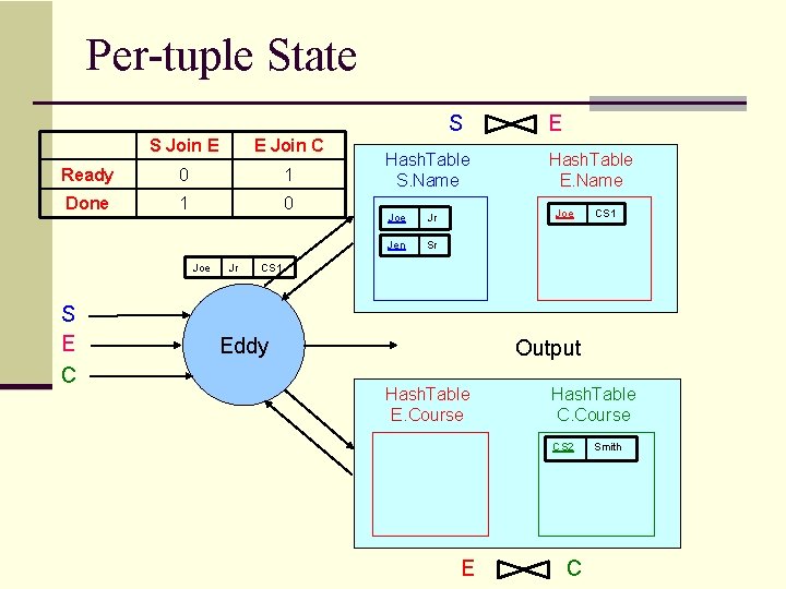
Per-tuple State n Here also we need to keep track of what operators a tuple has already been through n Again use Ready bits - operators that can be applied next n Done bits - operators that have already been applied n n Unlike selections, these are not bit- complements of each other

Per-tuple State S S Join E E Join C Ready 1 0 Done 0 0 Joe S E C Hash. Table S. Name E Hash. Table E. Name Junior Eddy Output Hash. Table E. Course E Hash. Table C. Course C

Per-tuple State S S Join E E Join C Ready 1 1 Done 0 0 S E C Joe CS 1 Hash. Table S. Name Joe Jr Jen Sr Eddy E Hash. Table E. Name Output Hash. Table E. Course Hash. Table C. Course CS 2 E C Smith

Per-tuple State S S Join E E Join C Ready 0 1 Done 1 0 Joe S E C Jr Hash. Table S. Name Joe Jr Jen Sr E Hash. Table E. Name Joe CS 1 Eddy Output Hash. Table E. Course Hash. Table C. Course CS 2 E C Smith

Execution Postmortem n Can we talk about what exactly the eddy did during the execution ? n Yes !

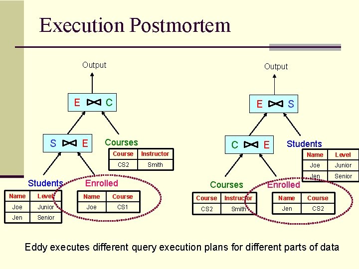
Execution Postmortem Output E S Students Output C E E Courses C S E Students Course Instructor Name Level CS 2 Smith Joe Junior Jen Senior Enrolled Courses Enrolled Name Level Name Course Instructor Name Course Joe Junior Joe CS 1 CS 2 Smith Jen CS 2 Jen Senior Eddy executes different query execution plans for different parts of data

Execution Postmortem n Can we talk about what exactly the eddy did during the execution ? n Yes ! n Eddy executes different plans for different parts of data n This is where the adaptivity comes from

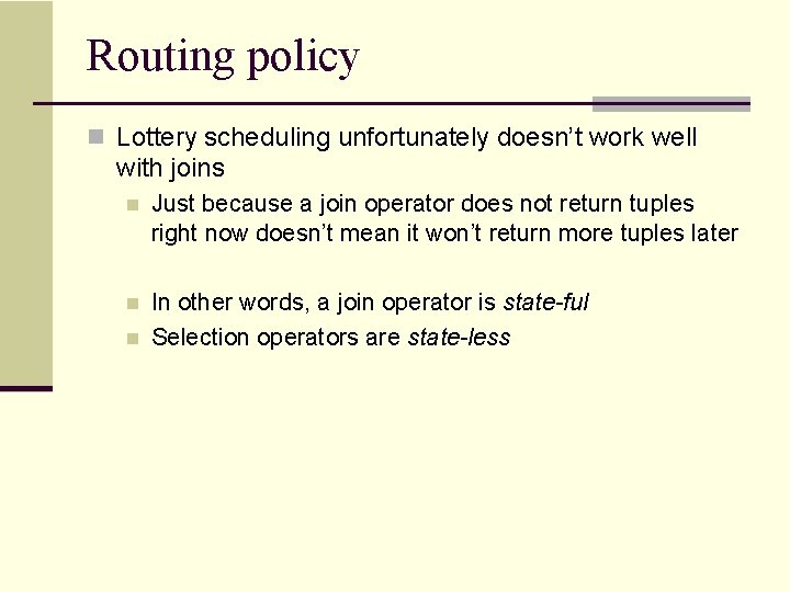
Routing policy n Lottery scheduling unfortunately doesn’t work well with joins n Just because a join operator does not return tuples right now doesn’t mean it won’t return more tuples later n In other words, a join operator is state-ful Selection operators are state-less n

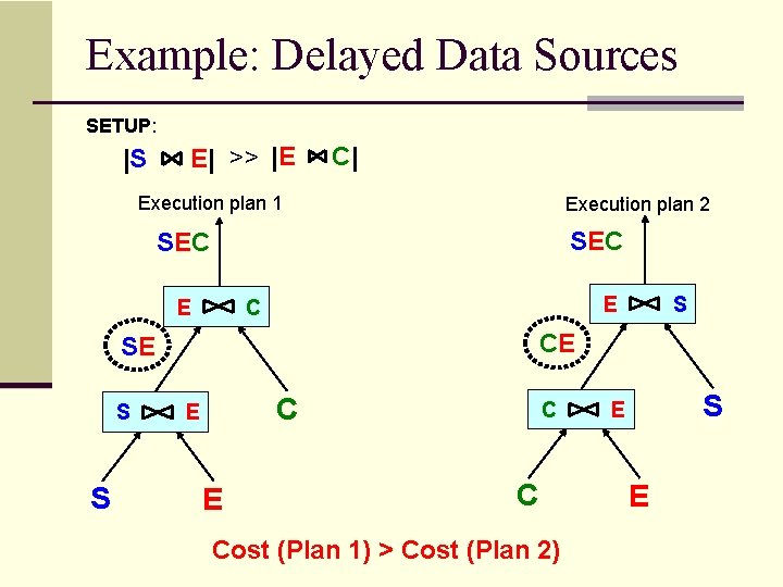
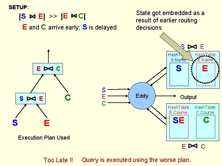
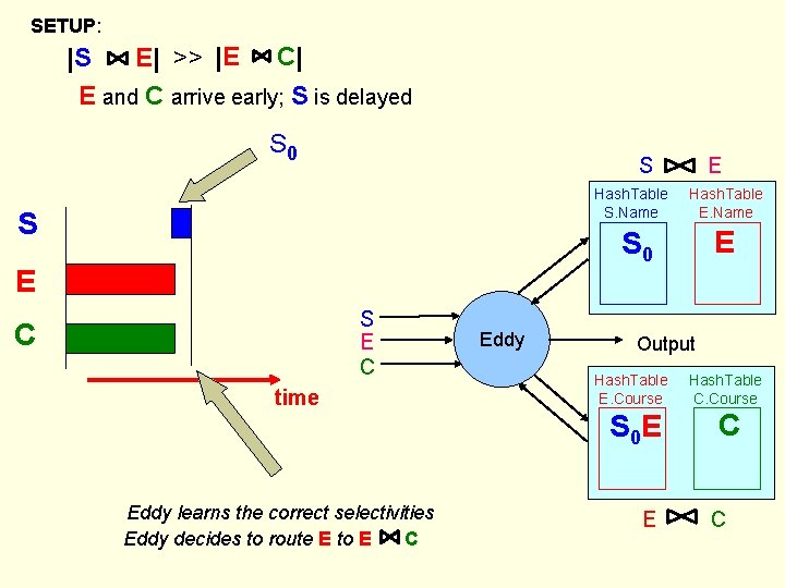
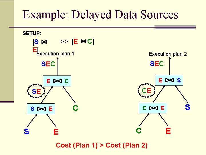
Example: Delayed Data Sources SETUP: |S E| >> |E C| Execution plan 1 Execution plan 2 SEC E E C CE SE S S S C E E C C Cost (Plan 1) > Cost (Plan 2) S E E

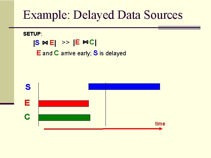
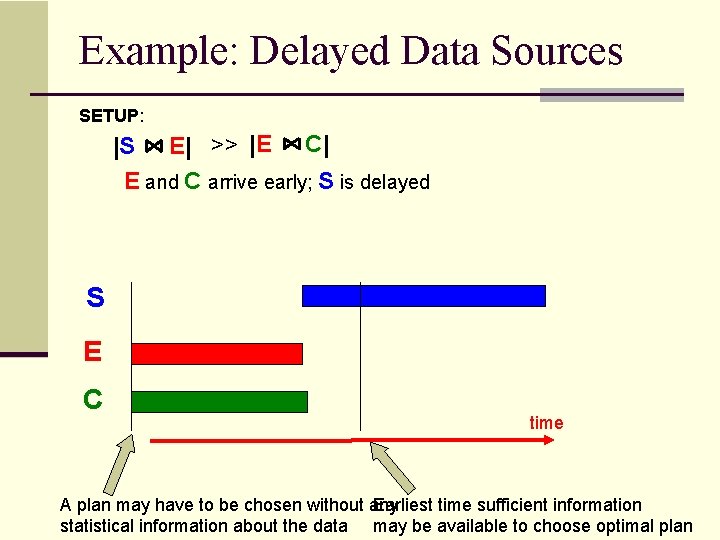
Example: Delayed Data Sources SETUP: |S E| >> |E C| E and C arrive early; S is delayed S E C time

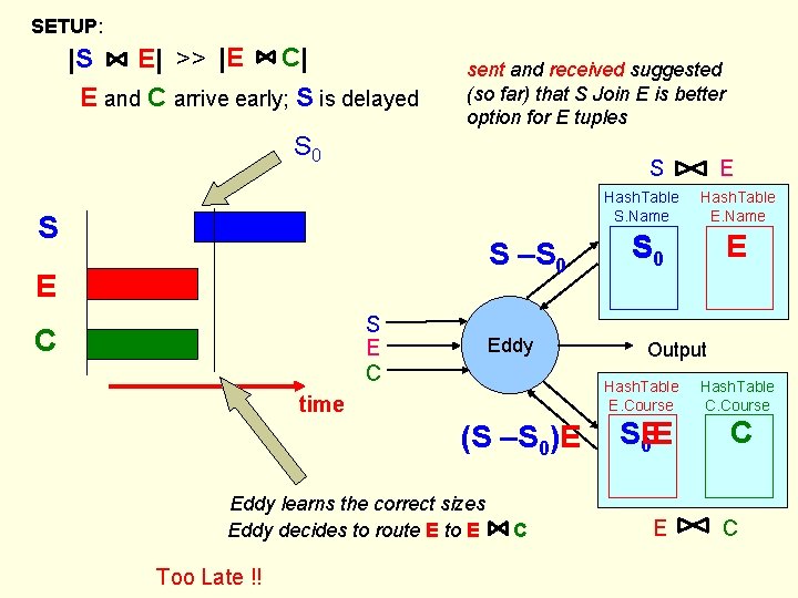
SETUP: |S E| >> |E C| E and C arrive early; S is delayed sent and received suggested (so far) that S Join E is better option for E tuples S 0 S Hash. Table S. Name S S –S 0 E S E C C Eddy (S –S 0)E Eddy learns the correct sizes Eddy decides to route E to E Too Late !! C Hash. Table E. Name S 0 E Output Hash. Table E. Course time E S 0 E SE E Hash. Table C. Course C C

SETUP: |S E| >> |E C| E and C arrive early; S is delayed State got embedded as a result of earlier routing decisions S E S S C C E E S E C Eddy E Hash. Table S. Name Hash. Table E. Name S E Output Hash. Table E. Course Hash. Table C. Course SE C Execution Plan Used E Too Late !! Query is executed using the worse plan. C

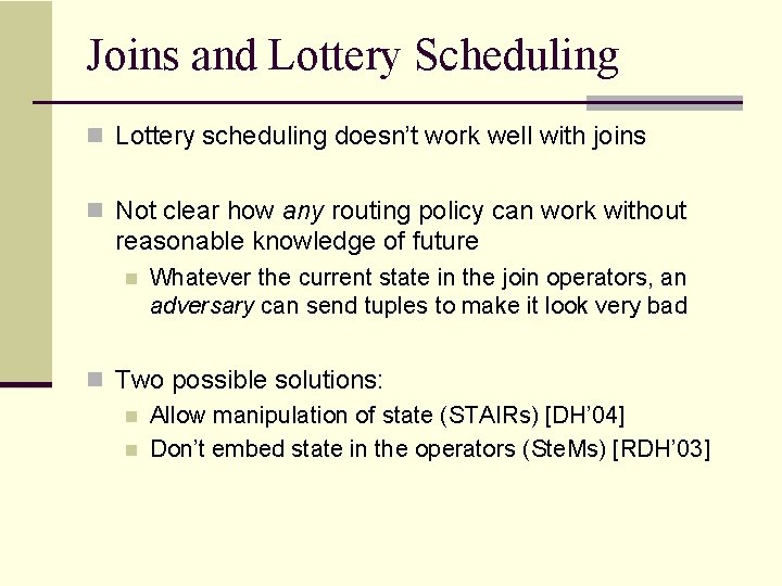
Joins and Lottery Scheduling n Lottery scheduling doesn’t work well with joins n Not clear how any routing policy can work without reasonable knowledge of future n Whatever the current state in the join operators, an adversary can send tuples to make it look very bad n Two possible solutions: n Allow manipulation of state (STAIRs) [DH’ 04] n Don’t embed state in the operators (Ste. Ms) [RDH’ 03]

Roadmap n Adaptive Query Processing: Motivation n Eddies [AH’ 00] n STAIRs [DH’ 04] and Ste. Ms [RDH’ 03] n Experimental Study n Implementation in Postgre. SQL [Des’ 03] n Continuous queries [MSHR’ 02] (very briefly) n Open problems

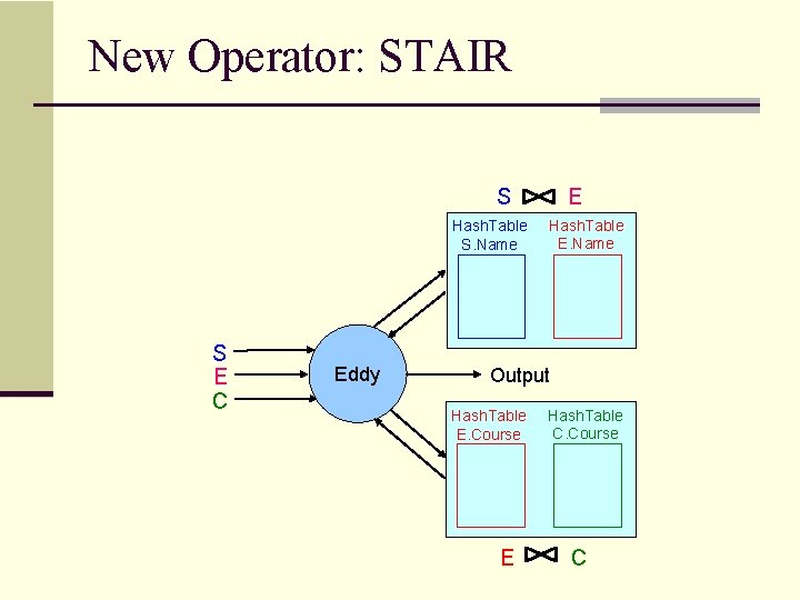
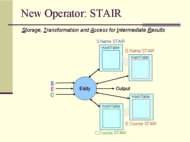
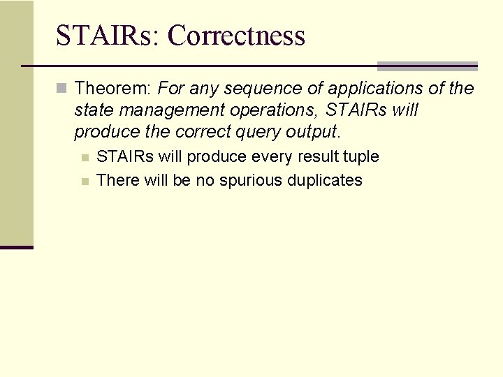
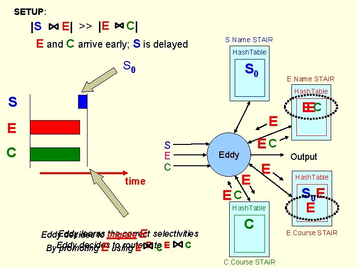
STAIRs [DH’ 04] n Expose join state to the eddy n Provide state management primitives n That guarantee correctness of execution n That can be used to manipulate embedded state in the operators n Also allow support for cyclic queries etc

New Operator: STAIR S Hash. Table S. Name S E C Eddy E Hash. Table E. Name Output Hash. Table E. Course E Hash. Table C. Course C

New Operator: STAIR Storage, Transformation and Access for Intermediate Results S. Name STAIR Hash. Table E. Name STAIR Hash. Table S E C Eddy Output Hash. Table E. Course STAIR C. Course STAIR

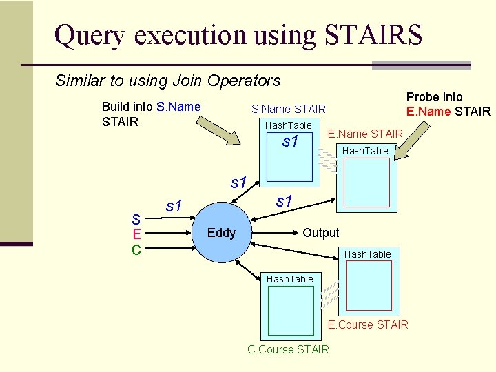
Query execution using STAIRS Similar to using Join Operators Build into S. Name STAIR Hash. Table s 1 S E C Probe into E. Name STAIR s 1 Eddy E. Name STAIR Hash. Table s 1 Output Hash. Table E. Course STAIR C. Course STAIR

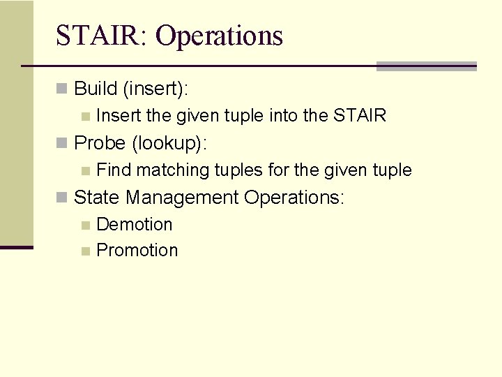
STAIR: Operations n Build (insert): n Insert the given tuple into the STAIR n Probe (lookup): n Find matching tuples for the given tuple n State Management Operations: n Demotion n Promotion

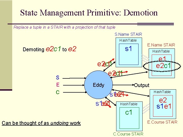
State Management Primitive: Demotion Replace a tuple in a STAIR with a projection of that tuple S. Name STAIR Hash. Table s 1 Demoting e 2 c 1 to e 2 S E C E. Name STAIR Hash. Table e 1 e 2 c 1 e 1 Eddy Output s 1 e 1 e 2 Hash. Table s 1 e 1 e 2 c 1 Hash. Table e 2 s 1 e 1 E. Course STAIR Can be thought of as undoing work C. Course STAIR

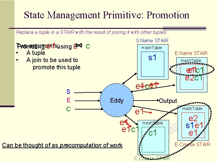
State Management Primitive: Promotion Replace a tuple in a STAIR with the result of joining it with other tuples S. Name STAIR Two arguments: Promoting e 1 using E C • A tuple • A join to be used to promote this tuple S E C Hash. Table E. Name STAIR s 1 Hash. Table e 1 c 1 e 2 c 1 e 1 c 1 Eddy Output Hash. Table e 1 e 1 c 1 Hash. Table c 1 e 2 s 1 e 1 E. Course STAIR Can be thought of as precomputation of work C. Course STAIR

STAIRs: Correctness n Theorem: For any sequence of applications of the state management operations, STAIRs will produce the correct query output. n n STAIRs will produce every result tuple There will be no spurious duplicates

Lifting Burden of History: Delayed Data Sources

SETUP: |S E| >> |E C| E and C arrive early; S is delayed S 0 S Hash. Table S. Name S E Hash. Table E. Name E S 0 E S E C C time Eddy learns the correct selectivities Eddy decides to route E to E C Eddy Output Hash. Table E. Course S 0 E E Hash. Table C. Course C C

SETUP: |S E| >> |E C| E and C arrive early; S is delayed S. Name STAIR Hash. Table S 0 E. Name STAIR Hash. Table S E E S E C C time EC Eddy E E EC Hash. Table learns the correct Eddy decides to migrate E selectivities decides to route C By. Eddy promoting E using E E to CE EEC C C. Course STAIR Output Hash. Table S 0 E E E. Course STAIR

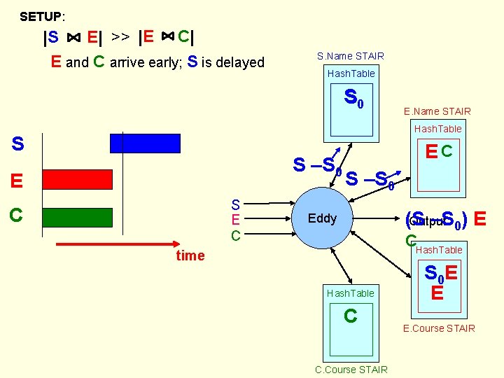
SETUP: |S E| >> |E C| E and C arrive early; S is delayed S. Name STAIR Hash. Table S 0 E. Name STAIR Hash. Table S S –S 0 E S E C C EC S –S 0 (S –S 0) E Output Eddy CHash. Table time Hash. Table C C. Course STAIR S 0 E E E. Course STAIR

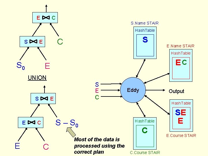
E C S. Name STAIR Hash. Table S S C E E. Name STAIR Hash. Table S 0 EC E UNION S E E S E C Output Hash. Table S – S 0 C Eddy Most of the data is processed using the correct plan Hash. Table C C. Course STAIR SE E E. Course STAIR

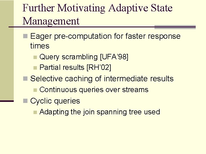
Further Motivating Adaptive State Management n Eager pre-computation for faster response times Query scrambling [UFA’ 98] n Partial results [RH’ 02] n n Selective caching of intermediate results n Continuous queries over streams n Cyclic queries n Adapting the join spanning tree used

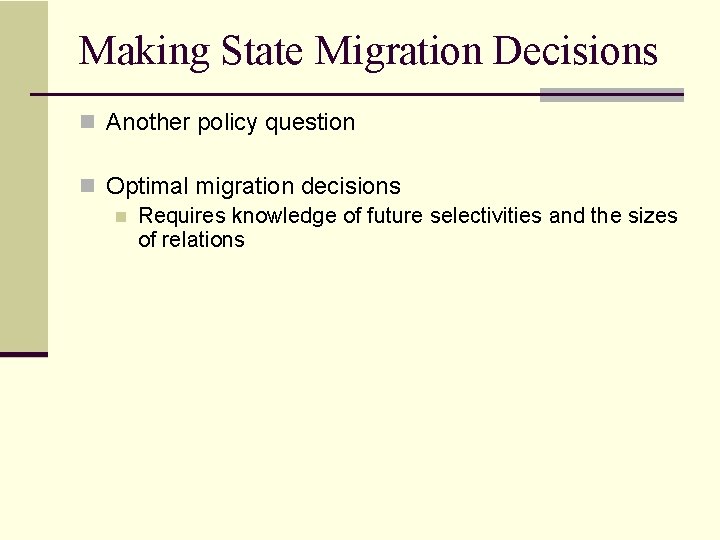
Making State Migration Decisions n Another policy question n Optimal migration decisions n Requires knowledge of future selectivities and the sizes of relations

Roadmap n Adaptive Query Processing: Motivation n Eddies [AH’ 00] n STAIRs [DH’ 04] and Ste. Ms [RDH’ 03] n Experimental Study n Implementation in Postgre. SQL [Des’ 03] n Continuous queries [MSHR’ 02] (very briefly) n Open problems

Alternative: Ste. Ms [RDH’ 03] n Don’t embed the state in the operators at all n Note: Not the original motivation for Ste. Ms n Focus was on increasing opportunities for adaptivity by breaking up the join operators n We will focus on a very simplistic version of the operator

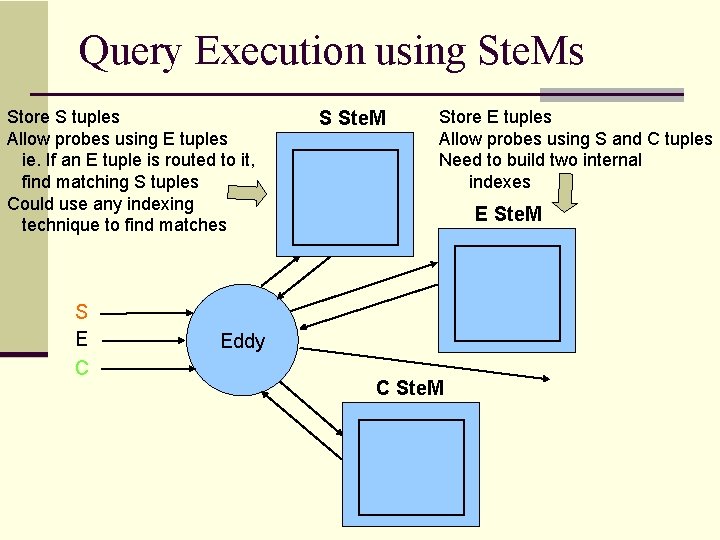
Query Execution using Ste. Ms Store S tuples Allow probes using E tuples ie. If an E tuple is routed to it, find matching S tuples Could use any indexing technique to find matches S E C S Ste. M Store E tuples Allow probes using S and C tuples Need to build two internal indexes E Ste. M Eddy C Ste. M

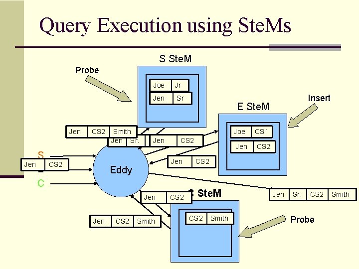
Query Execution using Ste. Ms S Ste. M Probe Jen S Jen E C CS 2 Smith Jen Sr. Joe Jr Jen Sr CS 2 Jen Smith CS 2 Eddy Jen CS 2 E Ste. M Joe Jen Smith CS 2 Insert Jen CS 1 CS 2 C Ste. M CS 2 Smith Jen Sr. CS 2 Probe Smith

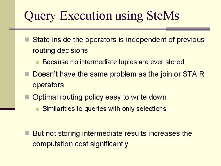
Query Execution using Ste. Ms n State inside the operators is independent of previous routing decisions n Because no intermediate tuples are ever stored n Doesn’t have the same problem as the join or STAIR operators n Optimal routing policy easy to write down n Similarities to queries with only selections n But not storing intermediate results increases the computation cost significantly

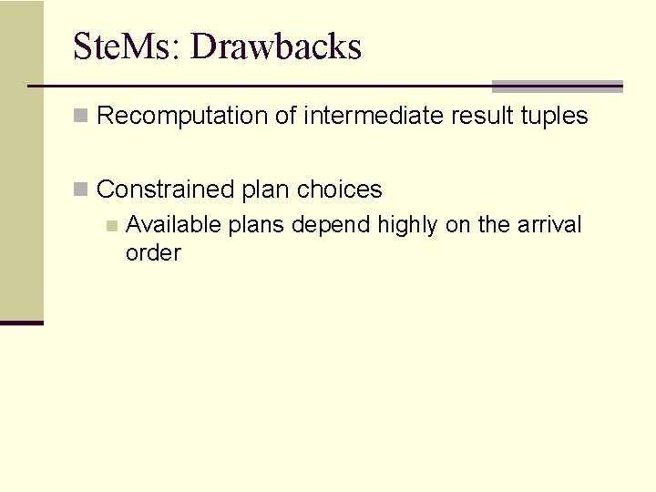
Ste. Ms: Drawbacks n Recomputation of intermediate result tuples n Constrained plan choices n Available plans depend highly on the arrival order

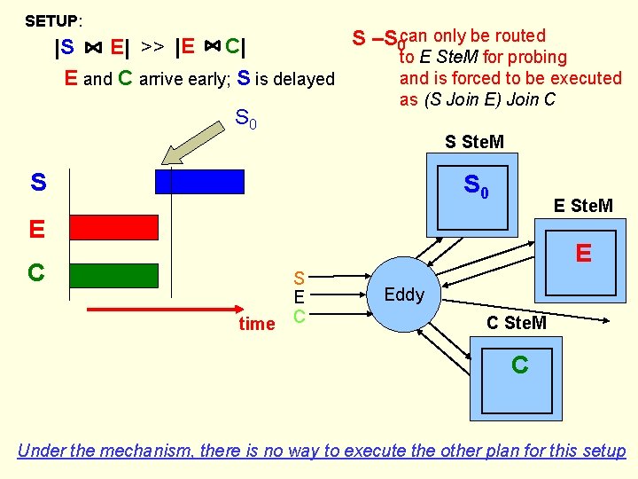
SETUP: can only be routed S –S 0 |E C| |S E| >> to E Ste. M for probing and is forced to be executed E and C arrive early; S is delayed as (S Join E) Join C S 0 S Ste. M S S 0 E Ste. M E E C time S E C Eddy C Ste. M C Under the mechanism, there is no way to execute the other plan for this setup

Ste. Ms: Drawbacks n Recomputation of intermediate result tuples n Constrained plan choices n Available plans depend highly on the arrival order n Though more subtle, the second drawback might be the more important one

Recap n An eddy operator n Can affect the query execution plan(s) used by routing different tuples differently n Eddy w/ Selections: n Well understood n Even if selections are correlated n Babu, Munagala et al [SIGMOD 2004, ICDT 2005]

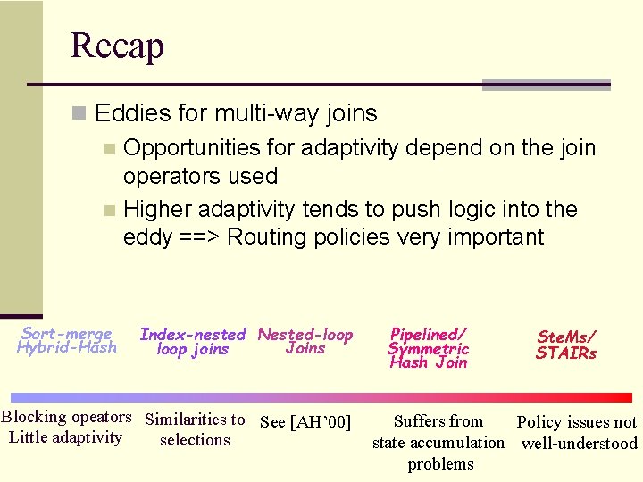
Recap n Eddies for multi-way joins n Opportunities for adaptivity depend on the join operators used n Higher adaptivity tends to push logic into the eddy ==> Routing policies very important Sort-merge Hybrid-Hash Index-nested Nested-loop Joins loop joins Blocking opeators Similarities to See [AH’ 00] Little adaptivity selections Pipelined/ Symmetric Hash Join Ste. Ms/ STAIRs Suffers from Policy issues not state accumulation well-understood problems

Roadmap n Adaptive Query Processing: Motivation n Eddies [AH’ 00] n STAIRs [DH’ 04] and Ste. Ms [RDH’ 03] n Experimental Study n Implementation in Postgre. SQL [Des’ 03] n Continuous queries [MSHR’ 02] (very briefly) n Open problems

Implementation Details n In Postgre. SQL Database System code base n In the context of Telegraph. CQ project n Highly efficient implementation [SIGREC’ 04] n Eddy, Ste. Ms, STAIRs export get_next() functions n Routing decisions are made per batch n n Can control batch size n Routing decisions made for all possible ready bitmaps Decisions are encoded in arrays that are indexed with ready bits n Efficiently find the operator to route to

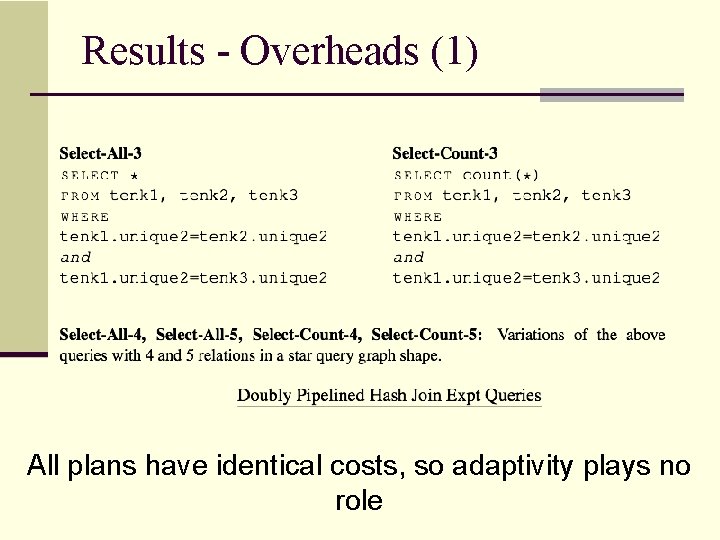
Results - Overheads (1) All plans have identical costs, so adaptivity plays no role

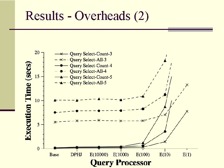
Results - Overheads (2)

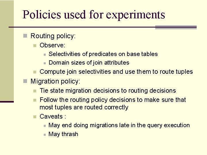
Policies used for experiments n Routing policy: n Observe: n Selectivities of predicates on base tables n Domain sizes of join attributes n Compute join selectivities and use them to route tuples n Migration policy: n Tie state migration decisions to routing decisions n Follow the routing policy decisions to make sure that most tuples are routed correctly n Caveats : n May end doing migrations late in the query execution n May thrash

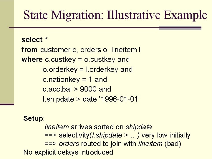
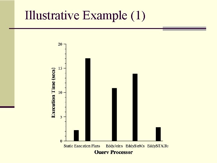
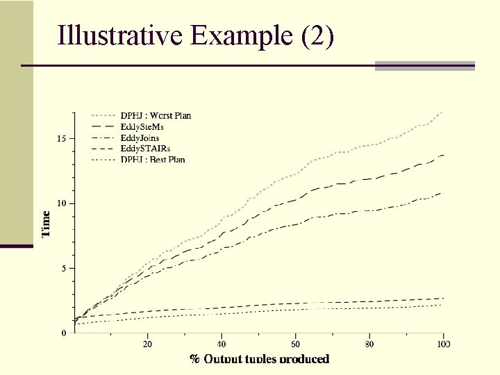
State Migration: Illustrative Example select * from customer c, orders o, lineitem l where c. custkey = o. custkey and o. orderkey = l. orderkey and c. nationkey = 1 and c. acctbal > 9000 and l. shipdate > date ’ 1996 -01 -01’ Setup: lineitem arrives sorted on shipdate ==> selectivity(l. shipdate > …) very low initially ==> orders routed to join with lineitem (bad) No explicit delays introduced

Illustrative Example (1)

Illustrative Example (2)

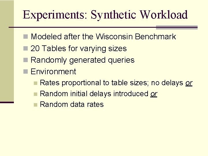
Experiments: Synthetic Workload n Modeled after the Wisconsin Benchmark n 20 Tables for varying sizes n Randomly generated queries n Environment n Rates proportional to table sizes; no delays or n Random initial delays introduced or n Random data rates

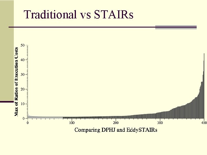
Traditional vs STAIRs

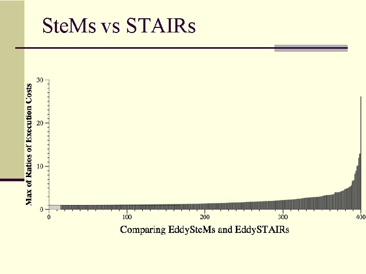
Ste. Ms vs STAIRs

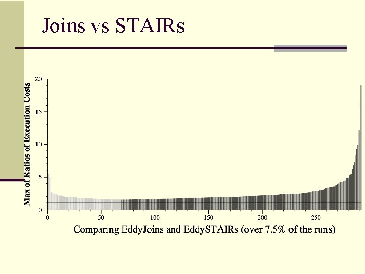
Joins vs STAIRs

Roadmap n Adaptive Query Processing: Motivation n Eddies [AH’ 00] n STAIRs [DH’ 04] and Ste. Ms [RDH’ 03] n Experimental Study n Implementation in Postgre. SQL [Des’ 03] n Continuous queries [MSHR’ 02] (very briefly) n Open problems

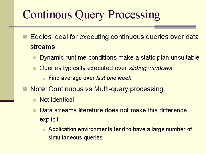
Continous Query Processing n Eddies ideal for executing continuous queries over data streams n Dynamic runtime conditions make a static plan unsuitable n Queries typically executed over sliding windows n Find average over last one week n Note: Continuous vs Multi-query processing n Not identical n Data streams literature does not make this difference explicit n Application environments tend to have a large number of simultaneous queries

Continuous Query Processing n CACQ [Madden et al 2002] n Focus on sharing work as much as adaptivity n Uses Ste. Ms augmented with a deletion operator n n To handle sliding windows Also uses predicate indexes n n For handling a large number of queries on the same set of streams but with different predicates E. g. millions of stock alerts over a few streams

Roadmap n Adaptive Query Processing: Motivation n Eddies [AH’ 00] n STAIRs [DH’ 04] and Ste. Ms [RDH’ 03] n Experimental Study n Implementation in Postgre. SQL [Des’ 03] n Continuous queries [MSHR’ 02] (very briefly) n Open problems

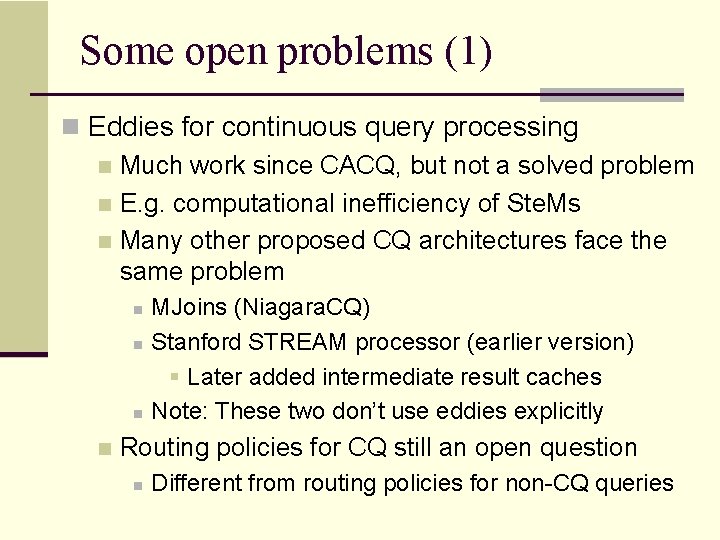
Some open problems (1) n Eddies for continuous query processing n Much work since CACQ, but not a solved problem n E. g. computational inefficiency of Ste. Ms n Many other proposed CQ architectures face the same problem n n MJoins (Niagara. CQ) Stanford STREAM processor (earlier version) § Later added intermediate result caches Note: These two don’t use eddies explicitly Routing policies for CQ still an open question n Different from routing policies for non-CQ queries

Some open problems (2) n Routing policies n Whether eddies will succeed depends on the routing policies n Little work so far. . . n Ste. Ms, STAIRs n Theoretical analysis of optimization space, and practical viability analysis needed n Especially in the context of continuous query processing

Some open problems (3) n Eddies for multi-query processing (non-CQ) n Ste. Ms may be sufficient for CQ processing, but not for normal multi-query processing n Parallel, distributed environments, P 2 P, Grid. . n Disk: n Flexibility demanded by adaptive techniques at odds against the careful scheduling typically done by DBMSs n n XJoins Very little work on understanding this

Some open problems (4) n Optimization with expanded plan space n Eddies can explore a plan space much larger than traditional plan space n They allow relations to be broken into pieces, with each piece executed separately Can we explore this plan space in a nonadaptive setting ? n Recent work on: n n n Conditional Planning [Deshpande et al, ICDE 2005] Content-based Routing [Babu et al, VLDB 2005]

Summary n Increasing need for adaptivity n Eddy: A highly adaptive query processor n Executes queries by routing tuples through operators n Ste. Ms, STAIRs n New operators proposed to handle problems with traditional join operators n Very promising especially for continuous and wide-area query processing n Exciting research lies ahead…

The End n Questions ?

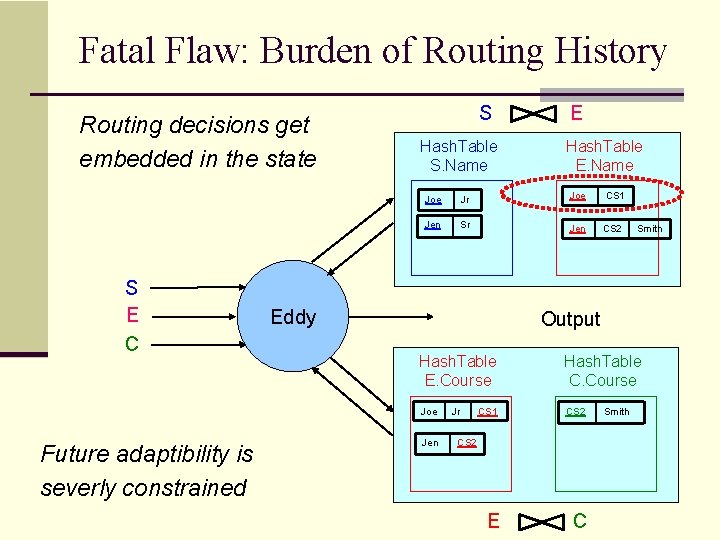
Fatal Flaw: Burden of Routing History Routing decisions get embedded in the state S E C Future adaptibility is severly constrained S Hash. Table S. Name E Hash. Table E. Name Joe Jr Joe CS 1 Jen Sr Jen CS 2 Eddy Smith Output Hash. Table E. Course Hash. Table C. Course Joe CS 2 Jen Jr CS 1 CS 2 E C Smith

Example: Delayed Data Sources SETUP: >> |E |S E|Execution plan 1 C| Execution plan 2 SEC E E C CE SE S S S C E E C C Cost (Plan 1) > Cost (Plan 2) S E E

Example: Delayed Data Sources SETUP: |S E| >> |E C| E and C arrive early; S is delayed S E C time A plan may have to be chosen without any Earliest time sufficient information statistical information about the data may be available to choose optimal plan

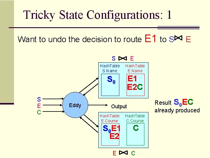
Tricky State Configurations: 1 Want to undo the decision to route E 1 to S S Hash. Table S. Name E Hash. Table E. Name E 1 E 2 C S 0 S E C Eddy Result S 0 EC already produced Output Hash. Table E. Course S 0 E 1 E 2 E E Hash. Table C. Course C C

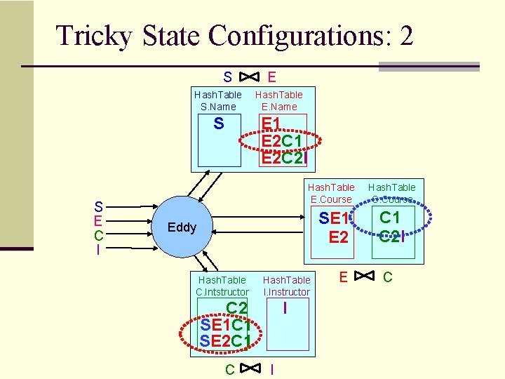
Tricky State Configurations: 2 S Hash. Table S. Name Hash. Table E. Name E 1 E 2 C 2 I S S E C I E Hash. Table E. Course SE 1 E 2 Eddy Hash. Table C. Intstructor Hash. Table I. Instructor C 2 SE 1 C 1 SE 2 C 1 C I I E Hash. Table C. Course C 1 C 2 I C