9 Protein Docking 1 Prediction of proteinprotein interactions

9. Protein Docking 1

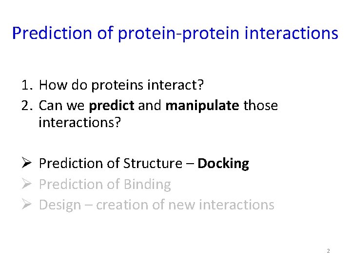
Prediction of protein-protein interactions 1. How do proteins interact? 2. Can we predict and manipulate those interactions? Ø Prediction of Structure – Docking Ø Prediction of Binding Ø Design – creation of new interactions 2

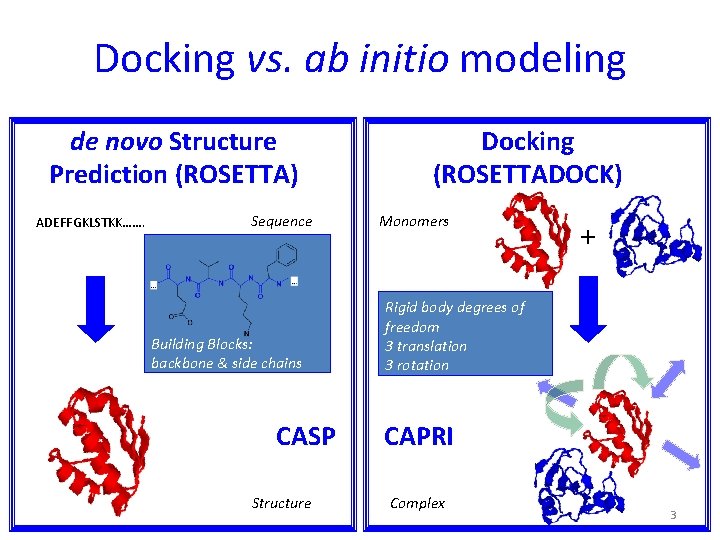
Docking vs. ab initio modeling de novo Structure Prediction (ROSETTA) ADEFFGKLSTKK……. Sequence Building Blocks: backbone & side chains CASP Structure Docking (ROSETTADOCK) Monomers + Rigid body degrees of freedom 3 translation 3 rotation CAPRI Complex 3

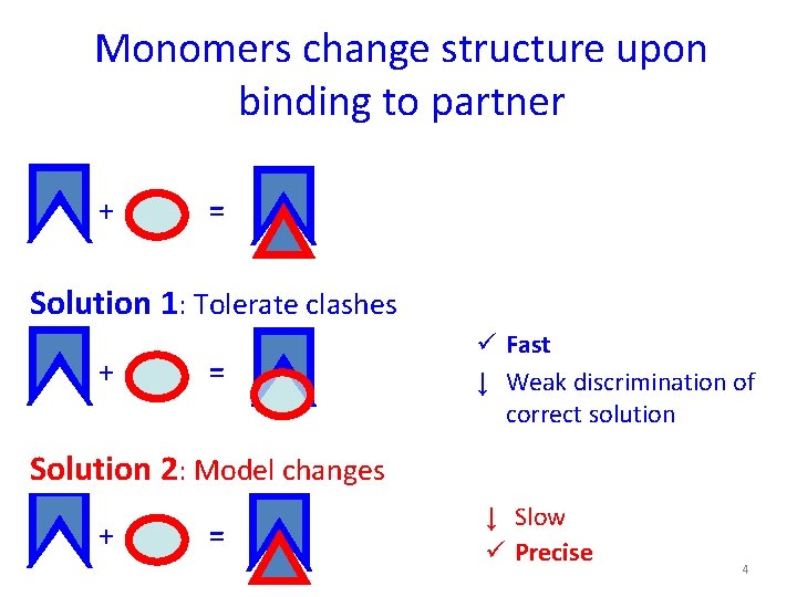
Monomers change structure upon binding to partner + = Solution 1: Tolerate clashes + = ü Fast ↓ Weak discrimination of correct solution Solution 2: Model changes + = ↓ Slow ü Precise 4

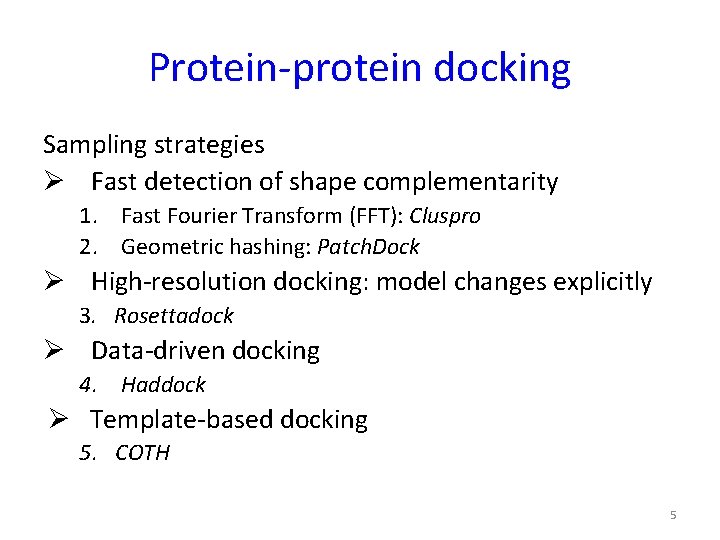
Protein-protein docking Sampling strategies Ø Fast detection of shape complementarity 1. Fast Fourier Transform (FFT): Cluspro 2. Geometric hashing: Patch. Dock Ø High-resolution docking: model changes explicitly 3. Rosettadock Ø Data-driven docking 4. Haddock Ø Template-based docking 5. COTH 5

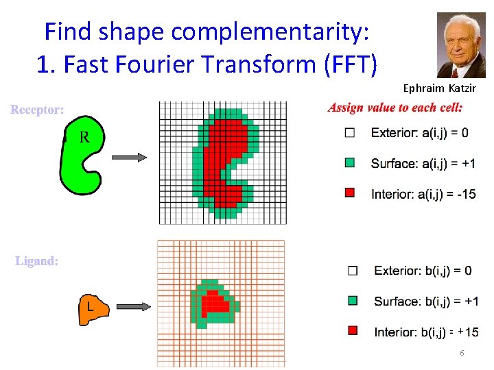
Find shape complementarity: 1. Fast Fourier Transform (FFT) Ephraim Katzir + 6

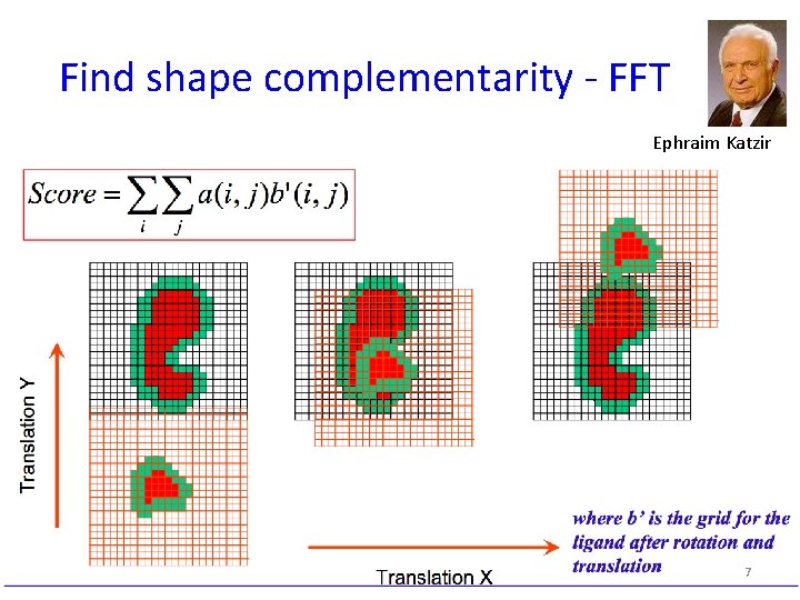
Find shape complementarity - FFT Ephraim Katzir 7

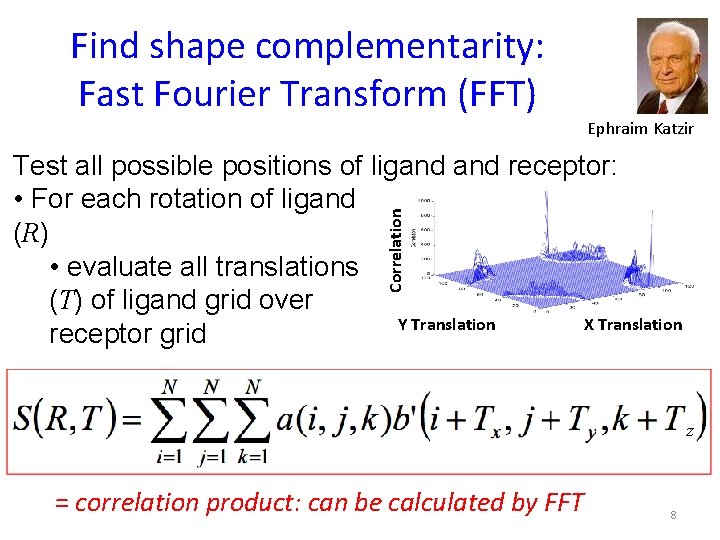
Find shape complementarity: Fast Fourier Transform (FFT) Ephraim Katzir Correlation Test all possible positions of ligand receptor: • For each rotation of ligand (R) • evaluate all translations (T) of ligand grid over Y Translation X Translation receptor grid z = correlation product: can be calculated by FFT 8

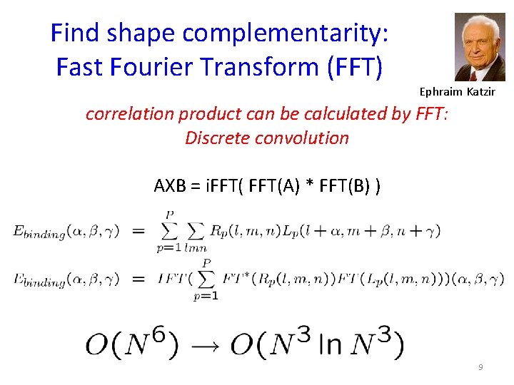
Find shape complementarity: Fast Fourier Transform (FFT) Ephraim Katzir correlation product can be calculated by FFT: Discrete convolution AXB = i. FFT(A) * FFT(B) ) 9

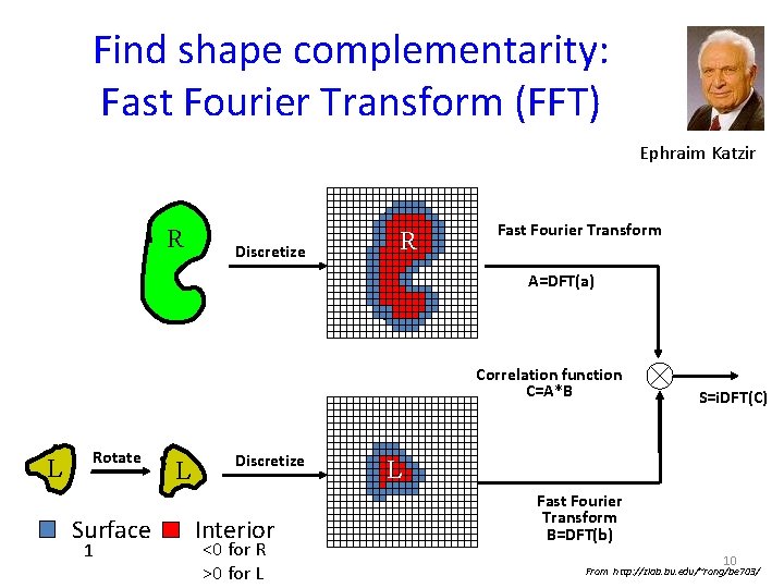
Find shape complementarity: Fast Fourier Transform (FFT) Ephraim Katzir R Discretize R R Fast Fourier Transform A=DFT(a) Correlation function C=A*B L Rotate Surface 1 L Discretize Interior <0 for R >0 for L S=i. DFT(C) L Fast Fourier Transform B=DFT(b) 10 From http: //zlab. bu. edu/~rong/be 703/

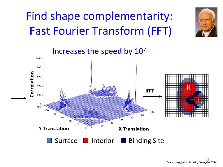
Find shape complementarity: Fast Fourier Transform (FFT) Correlation Increases the speed by 107 IFFT R L Y Translation Surface X Translation Interior Binding Site 11 From http: //zlab. bu. edu/~rong/be 703/

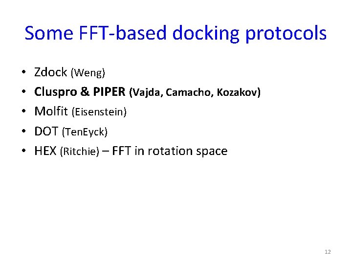
Some FFT-based docking protocols • • • Zdock (Weng) Cluspro & PIPER (Vajda, Camacho, Kozakov) Molfit (Eisenstein) DOT (Ten. Eyck) HEX (Ritchie) – FFT in rotation space 12

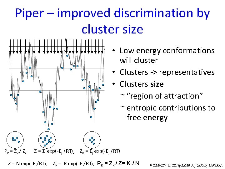
Piper – improved discrimination by cluster size • Low energy conformations will cluster • Clusters -> representatives • Clusters size ~ “region of attraction” ~ entropic contributions to free energy Pk = Zk / Z, Z = Σj exp(-Ej /RT), Zk = Σj exp(-Ej /RT) Z = N exp(-E /RT), Zk = K exp(-E /RT), Pk = Zk / Z= K / N Kozakov Biophysical J. , 2005, 89: 867.

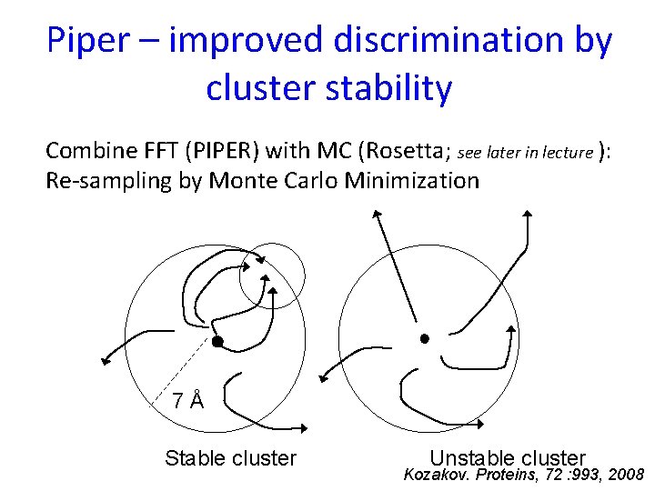
Piper – improved discrimination by cluster stability Combine FFT (PIPER) with MC (Rosetta; see later in lecture ): Re-sampling by Monte Carlo Minimization 7Å Stable cluster Unstable cluster Kozakov. Proteins, 72 : 993, 2008

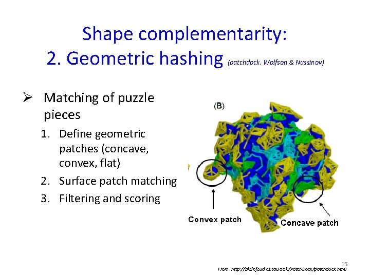
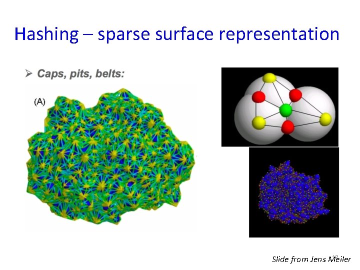
Shape complementarity: 2. Geometric hashing (patchdock, Wolfson & Nussinov) Ø Matching of puzzle pieces 1. Define geometric patches (concave, convex, flat) 2. Surface patch matching 3. Filtering and scoring 15 From http: //bioinfo 3 d. cs. tau. ac. il/Patch. Dock/patchdock. html

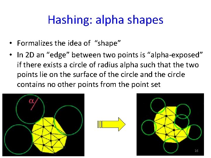
Hashing: alpha shapes • Formalizes the idea of “shape” • In 2 D an “edge” between two points is “alpha-exposed” if there exists a circle of radius alpha such that the two points lie on the surface of the circle and the circle contains no other points from the point set 16

Hashing – sparse surface representation 17 Slide from Jens Meiler

Docking with geometric hashing PATCHDOCK (by Dina Schneidmann ) • Fast and versatile approach • Speed allows easy extension to multiple protein docking, flexible hinge docking, etc • A extension of this protocol, FIREDOCK, includes side chain optimization (Rosetta. Docklike) – very flexible, fast and accurate protocol 18

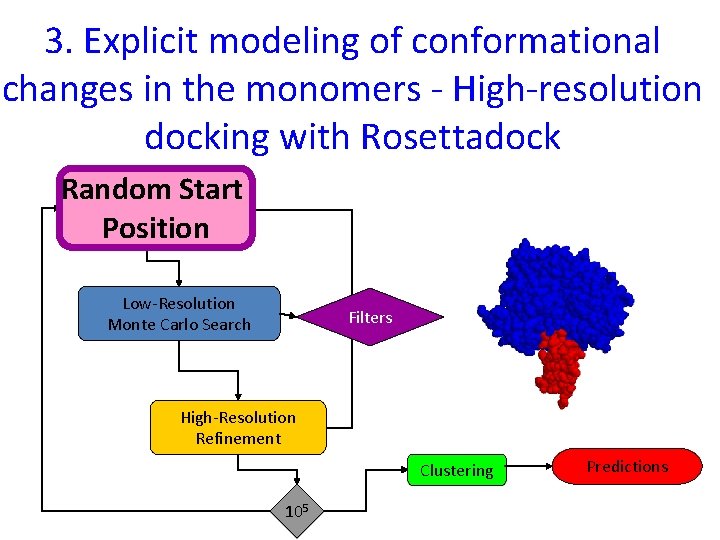
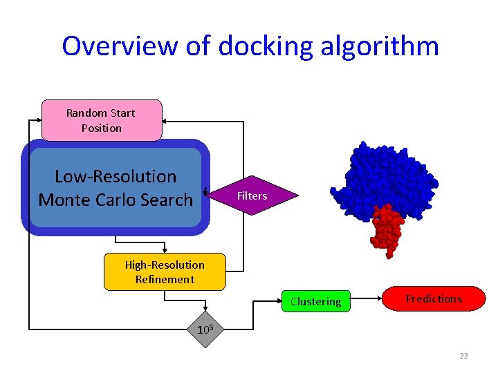
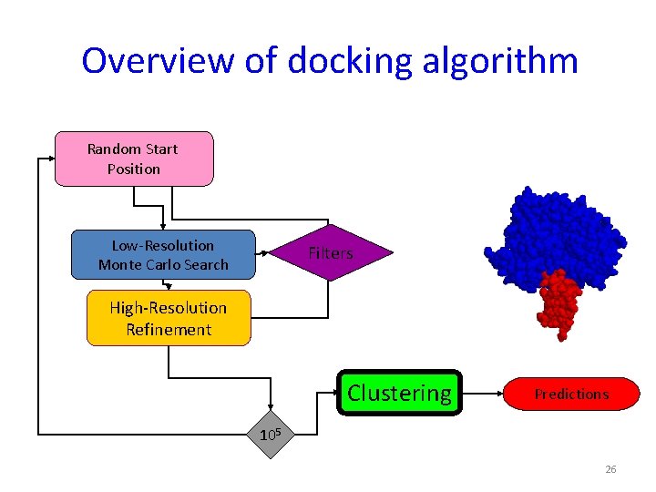
3. Explicit modeling of conformational changes in the monomers - High-resolution docking with Rosettadock Random Start Position Low-Resolution Monte Carlo Search Filters High-Resolution Refinement Clustering 105 Predictions

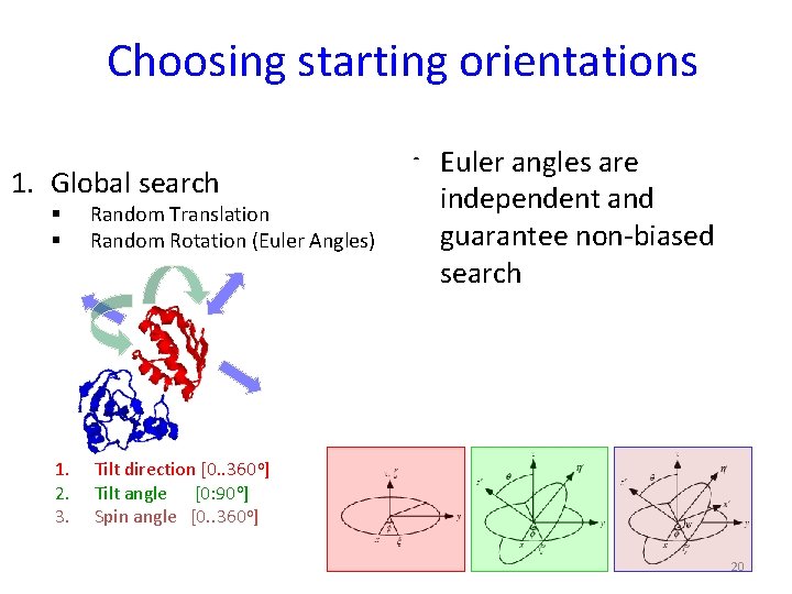
Choosing starting orientations 1. Global search § § Random Translation Random Rotation (Euler Angles) 1. 2. 3. Tilt direction [0. . 360 o] Tilt angle [0: 90 o] Spin angle [0. . 360 o] • Euler angles are independent and guarantee non-biased search 20

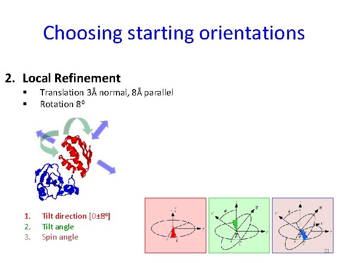
Choosing starting orientations 2. Local Refinement § § Translation 3Å normal, 8Å parallel Rotation 80 1. 2. 3. Tilt direction [0± 8 o] Tilt angle Spin angle 21

Overview of docking algorithm Random Start Position Low-Resolution Monte Carlo Search Filters High-Resolution Refinement Clustering Predictions 105 22

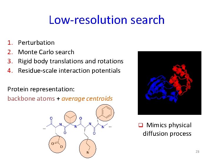
Low-resolution search 1. 2. 3. 4. Perturbation Monte Carlo search Rigid body translations and rotations Residue-scale interaction potentials Protein representation: backbone atoms + average centroids q Mimics physical diffusion process 23

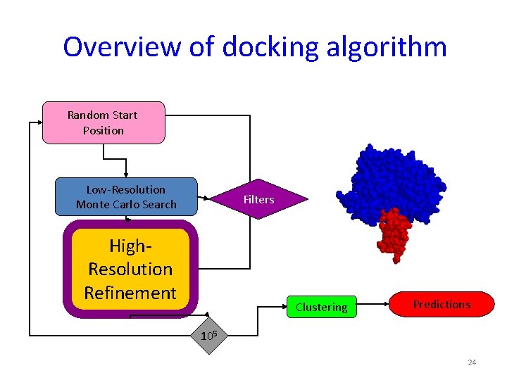
Overview of docking algorithm Random Start Position Low-Resolution Monte Carlo Search Filters High. Resolution Refinement Clustering Predictions 105 24

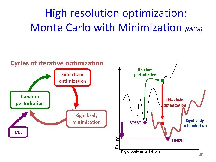
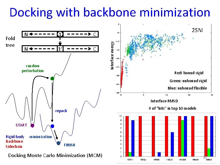
High resolution optimization: Monte Carlo with Minimization (MCM) Cycles of iterative optimization Random perturbation Side chain optimization Rigid body minimization START Energy MC FINISH Rigid body orientations 25

Overview of docking algorithm Random Start Position Low-Resolution Monte Carlo Search Filters High-Resolution Refinement Clustering Predictions 105 26

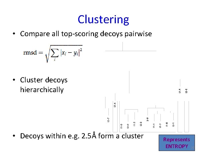
Clustering • Compare all top-scoring decoys pairwise • Cluster decoys hierarchically • Decoys within e. g. 2. 5Å form a cluster Represents ENTROPY 27

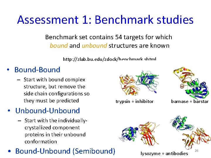
Assessment 1: Benchmark studies Benchmark set contains 54 targets for which bound and unbound structures are known http: //zlab. bu. edu/zdock/benchmark. shtml • Bound-Bound – Start with bound complex structure, but remove the side chain configurations so they must be predicted trypsin + inhibitor barnase + barstar • Unbound-Unbound – Start with the individuallycrystallized component proteins in their unbound conformation • Bound-Unbound (Semibound) lysozyme + antibodies 28

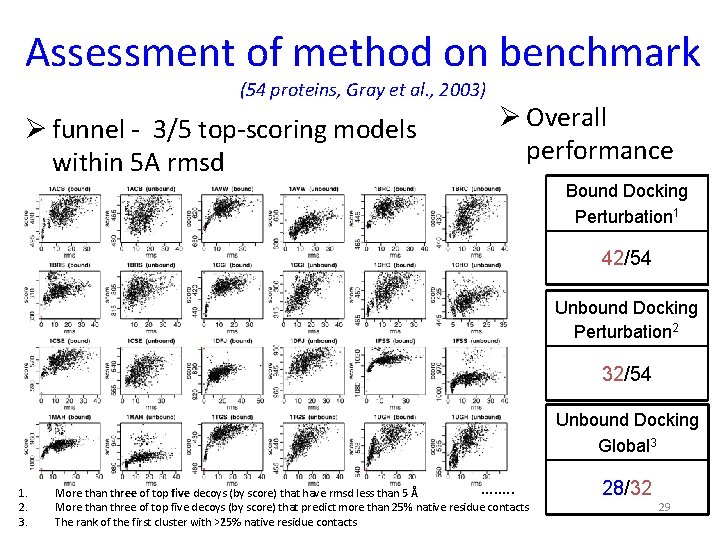
Assessment of method on benchmark (54 proteins, Gray et al. , 2003) Ø funnel - 3/5 top-scoring models within 5 A rmsd Ø Overall performance Bound Docking Perturbation 1 42/54 Unbound Docking Perturbation 2 32/54 Unbound Docking Global 3 1. 2. 3. ……. . More than three of top five decoys (by score) that have rmsd less than 5 Å More than three of top five decoys (by score) that predict more than 25% native residue contacts The rank of the first cluster with >25% native residue contacts 28/32 29

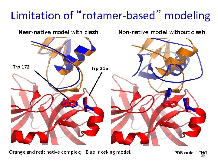
Limitation of “rotamer-based” modeling Near-native model with clash Trp 172 Non-native model without clash Trp 215 Orange and red: native complex; Blue: docking model. PDB code: 1 CHO 30

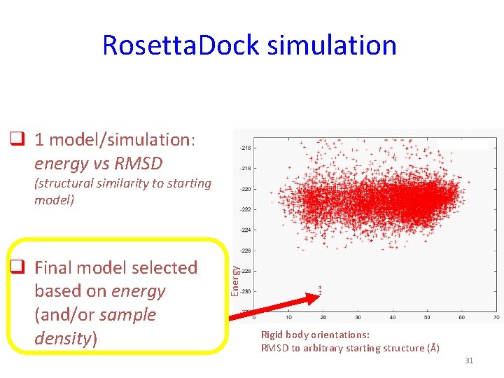
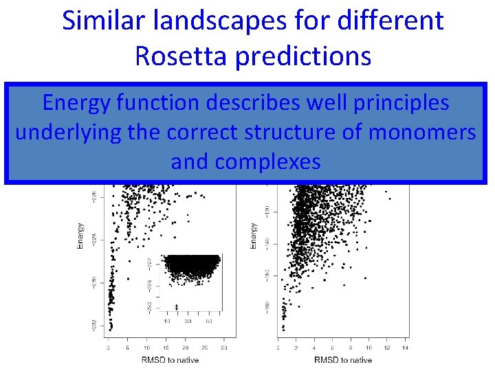
Rosetta. Dock simulation q 1 model/simulation: energy vs RMSD q Final model selected based on energy (and/or sample density) Energy (structural similarity to starting model) Rigid body orientations: RMSD to arbitrary starting structure (Å) 31

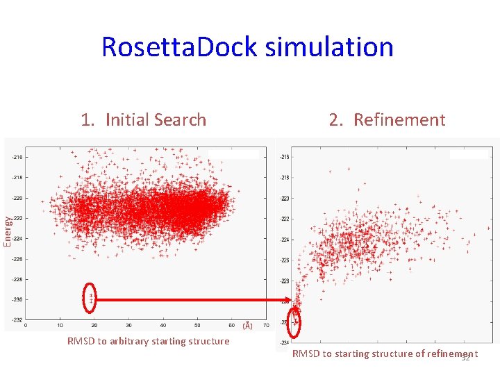
Rosetta. Dock simulation 2. Refinement Energy 1. Initial Search (Å) RMSD to arbitrary starting structure RMSD to starting structure of refinement 32

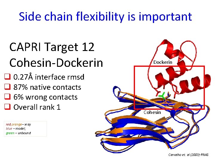
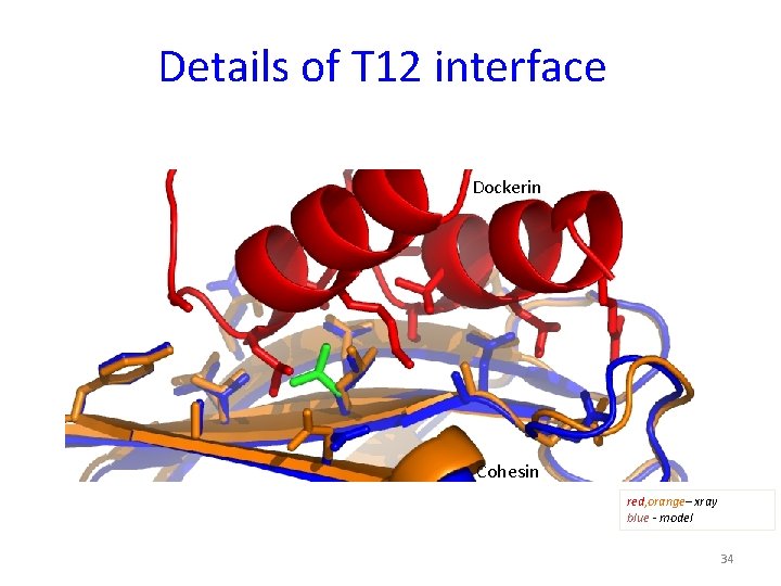
Side chain flexibility is important CAPRI Target 12 Cohesin-Dockerin q 0. 27Å interface rmsd q 87% native contacts q 6% wrong contacts q Overall rank 1 Dockerin Cohesin red, orange– xray blue – model; green – unbound Carvalho et. al (2003)33 PNAS

Details of T 12 interface Dockerin Cohesin red, orange– xray blue - model 34

Similar landscapes for different Rosetta predictions Docking Folding Energy function describes well principles energy landscape underlying the correct structure of monomers and complexes

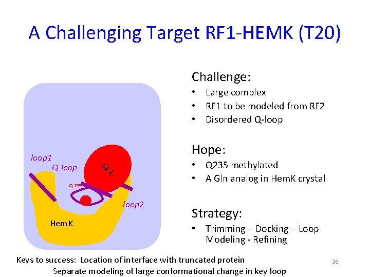
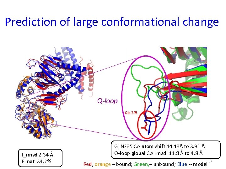
A Challenging Target RF 1 -HEMK (T 20) Challenge: RF 1 Q-loop Q 252 loop 1 Q-loop 2 RF loop 2 1 Q-235 loop 2 Hem. K • Large complex • RF 1 to be modeled from RF 2 • Disordered Q-loop Hope: • Q 235 methylated • A Gln analog in Hem. K crystal Strategy: • Trimming – Docking – Loop Modeling - Refining Keys to success: Location of interface with truncated protein Separate modeling of large conformational change in key loop 36

Prediction of large conformational change Gln 235 I_rmsd 2. 34 Ǻ F_nat 34. 2% GLN 235 C atom shift: 14. 13Ǻ to 3. 91 Ǻ Q-loop global C rmsd: 11. 8 Ǻ to 4. 8 Ǻ Red, orange – bound; Green, – unbound; Blue -- model 37

Docking with backbone minimization 1 C N 1’ C random perturbation 2 SNI Interface energy Fold tree N Red: bound rigid Green: unbound rigid Blue: unbound flexible Interface RMSD repack # of “hits” in top 10 models START Rigid-body Backbone Sidechain minimization FINISH Docking Monte Carlo Minimization (MCM) 38

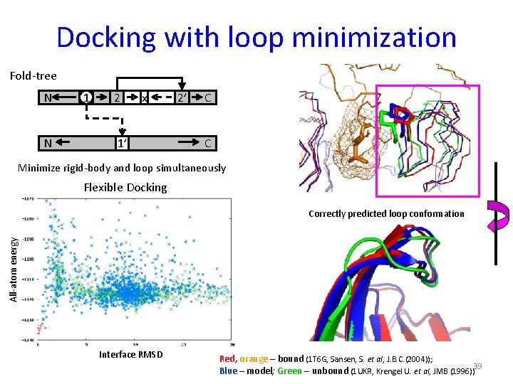
Docking with loop minimization Fold-tree N N 1 2 x 1’ 2’ C C Minimize rigid-body and loop simultaneously Flexible Docking All-atom energy Correctly predicted loop conformation Interface RMSD Red, orange – bound (1 T 6 G, Sansen, S. et al, J. B. C. (2004)); Blue – model; Green – unbound (1 UKR, Krengel U. et al, JMB (1996))39

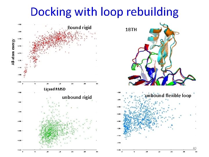
Docking with loop rebuilding 1 BTH All-atom energy Bound rigid Ligand RMSD unbound rigid unbound flexible loop 40

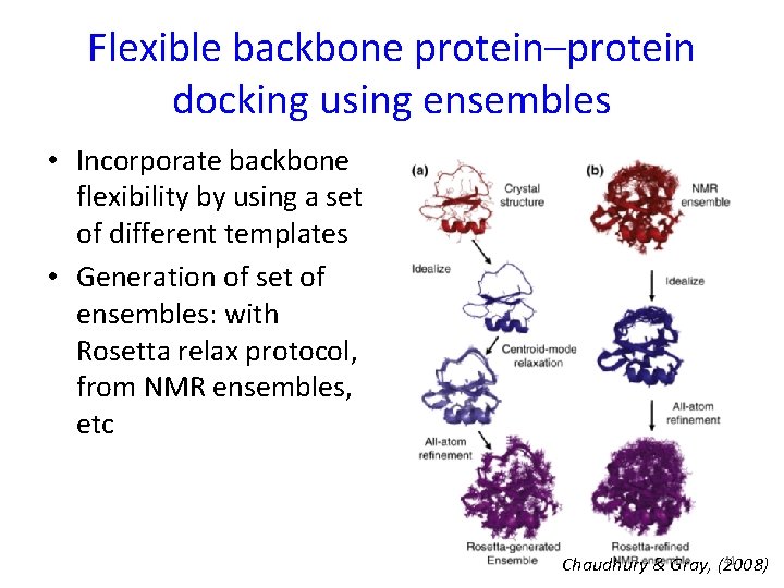
Flexible backbone protein–protein docking using ensembles • Incorporate backbone flexibility by using a set of different templates • Generation of set of ensembles: with Rosetta relax protocol, from NMR ensembles, etc 41 Chaudhury & Gray, (2008)

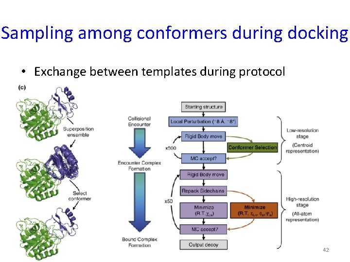
Sampling among conformers during docking • Exchange between templates during protocol 42

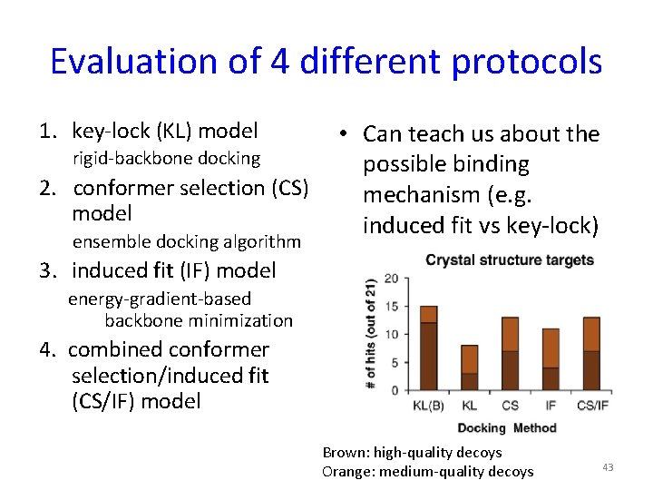
Evaluation of 4 different protocols 1. key-lock (KL) model rigid-backbone docking 2. conformer selection (CS) model ensemble docking algorithm • Can teach us about the possible binding mechanism (e. g. induced fit vs key-lock) 3. induced fit (IF) model energy-gradient-based backbone minimization 4. combined conformer selection/induced fit (CS/IF) model Brown: high-quality decoys Orange: medium-quality decoys 43

Rosetta. Dock 4. 0 Improvement due to better sampling and scoring: • Adaptive conformer selection (ACS): – Ensemble docking: conformer swapping rate adapted (few/many acceptances more/less sampling) • Replace low-resolution centroid score with Motif-Dock Score (MDS, using residue-pair transform score, RPX): – Parameters: aa 1, aa 2, 6 D transformation for superimposing N – Cα–C backbone atoms onto each other (for Cα < 10 A) – Lookup in pre-tabulated database Marze et al. Bioinformatics 2018

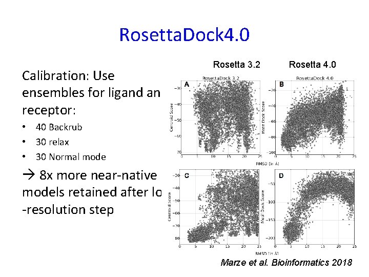
Rosetta. Dock 4. 0 Calibration: Use ensembles for ligand receptor: Rosetta 3. 2 Rosetta 4. 0 • 40 Backrub • 30 relax • 30 Normal mode 8 x more near-native models retained after low -resolution step Marze et al. Bioinformatics 2018

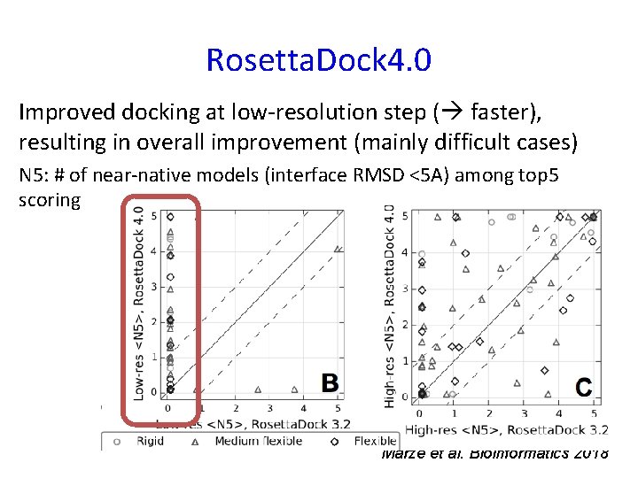
Rosetta. Dock 4. 0 Improved docking at low-resolution step ( faster), resulting in overall improvement (mainly difficult cases) N 5: # of near-native models (interface RMSD <5 A) among top 5 scoring Marze et al. Bioinformatics 2018

Rosetta. Dock - summary • First program to introduce general (side chain) flexibility during docking • Advanced the docking field towards unbiased high-resolution modeling • Many other protocols have since then incorporated Rosetta. Dock as a high-resolution final step • Targeted introduction of backbone flexibility can improve modeling dramatically 47

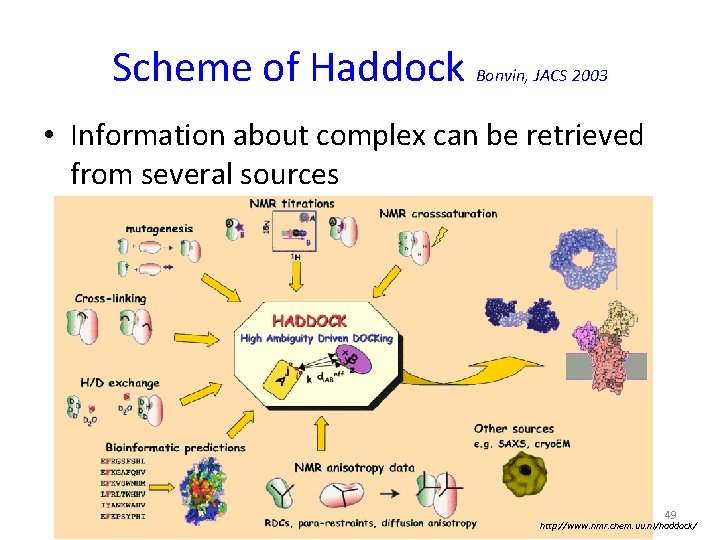
4. Data-driven docking • Challenges: – Large conformational space to sample – Conformational changes of proteins upon binding • Approach: restrict search space by previous information – HADDOCK (High Ambiguity Driven protein-protein Docking) 48

Scheme of Haddock Bonvin, JACS 2003 • Information about complex can be retrieved from several sources 49 http: //www. nmr. chem. uu. nl/haddock/

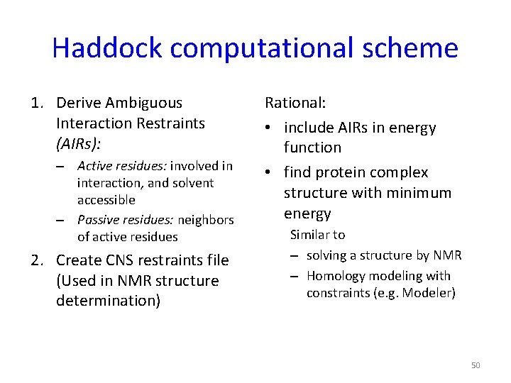
Haddock computational scheme 1. Derive Ambiguous Interaction Restraints (AIRs): – Active residues: involved in interaction, and solvent accessible – Passive residues: neighbors of active residues 2. Create CNS restraints file (Used in NMR structure determination) Rational: • include AIRs in energy function • find protein complex structure with minimum energy Similar to – solving a structure by NMR – Homology modeling with constraints (e. g. Modeler) 50

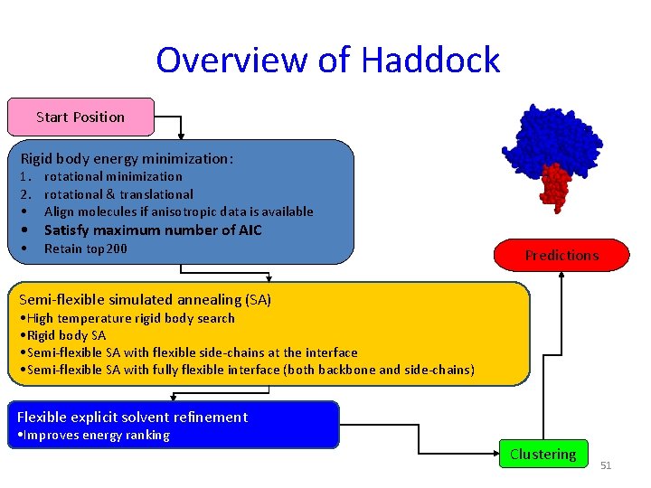
Overview of Haddock Start Position Rigid body energy minimization: 1. rotational minimization 2. rotational & translational • Align molecules if anisotropic data is available • Satisfy maximum number of AIC • Retain top 200 Predictions Semi-flexible simulated annealing (SA) • High temperature rigid body search • Rigid body SA • Semi-flexible SA with flexible side-chains at the interface • Semi-flexible SA with fully flexible interface (both backbone and side-chains) Flexible explicit solvent refinement • Improves energy ranking Clustering 51

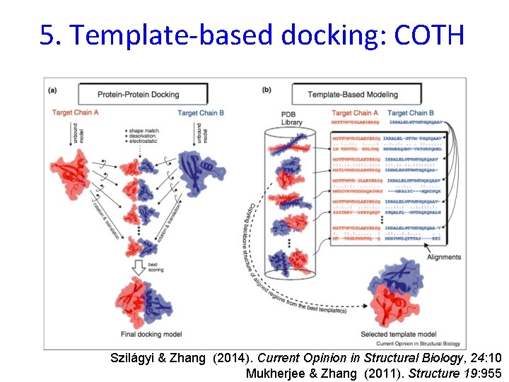
5. Template-based docking: COTH Szilágyi & Zhang (2014). Current Opinion in Structural Biology, 24: 10 Mukherjee & Zhang (2011). Structure 19: 955

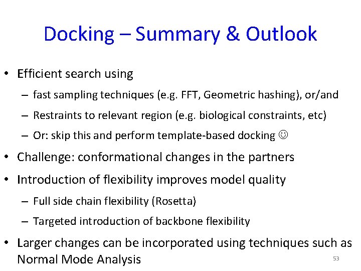
Docking – Summary & Outlook • Efficient search using – fast sampling techniques (e. g. FFT, Geometric hashing), or/and – Restraints to relevant region (e. g. biological constraints, etc) – Or: skip this and perform template-based docking • Challenge: conformational changes in the partners • Introduction of flexibility improves model quality – Full side chain flexibility (Rosetta) – Targeted introduction of backbone flexibility • Larger changes can be incorporated using techniques such as 53 Normal Mode Analysis