6 Point Estimation Copyright Cengage Learning All rights

6 Point Estimation Copyright © Cengage Learning. All rights reserved.

6. 1 Some General Concepts of Point Estimation Copyright © Cengage Learning. All rights reserved.

Some General Concepts of Point Estimation Statistical inference is almost always directed toward drawing some type of conclusion about one or more parameters (population characteristics). To do so requires that an investigator obtain sample data from each of the populations under study. Conclusions can then be based on the computed values of various sample quantities. For example, let (a parameter) denote the true average breaking strength of wire connections used in bonding semiconductor wafers. 3

Some General Concepts of Point Estimation A random sample of n = 10 connections might be made, and the breaking strength of each one determined, resulting in observed strengths x 1, x 2, . . . , x 10. The sample mean breaking strength x could then be used to draw a conclusion about the value of . Similarly, if 2 is the variance of the breaking strength distribution (population variance, another parameter), the value of the sample variance s 2 can be used to infer something about 2. 4

Some General Concepts of Point Estimation When discussing general concepts and methods of inference, it is convenient to have a generic symbol for the parameter of interest. We will use the Greek letter for this purpose. The objective of point estimation is to select a single number, based on sample data, that represents a sensible value for . As an example, the parameter of interest might be , the true average lifetime of batteries of a certain type. 5

Some General Concepts of Point Estimation A random sample of n = 3 batteries might yield observed lifetimes (hours) x 1 = 5. 0, x 2 = 6. 4, x 3 = 5. 9. The computed value of the sample mean lifetime is x = 5. 77, and it is reasonable to regard 5. 77 as a very plausible value of — our “best guess” for the value of based on the available sample information. Suppose we want to estimate a parameter of a single population (e. g. , or ) based on a random sample of size n. 6

Some General Concepts of Point Estimation We know that before data is available, the sample observations must be considered random variables (rv’s) X 1, X 2, . . . , X n. It follows that any function of the Xi ’s—that is, any statistic —such as the sample mean X or sample standard deviation S is also a random variable. The same is true if available data consists of more than one sample. For example, we can represent tensile strengths of m type 1 specimens and n type 2 specimens by X 1, . . . , Xm and Y 1, . . . , Yn, respectively. 7

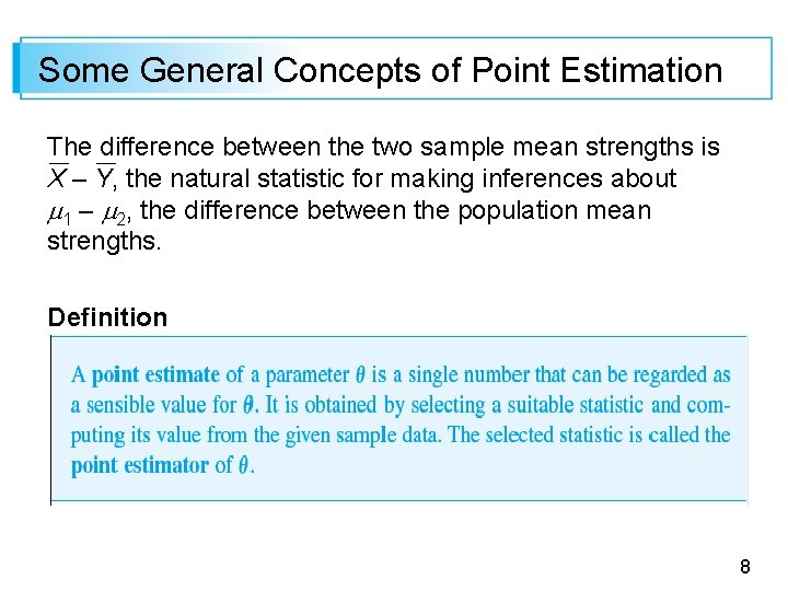
Some General Concepts of Point Estimation The difference between the two sample mean strengths is X – Y, the natural statistic for making inferences about 1 – 2, the difference between the population mean strengths. Definition 8

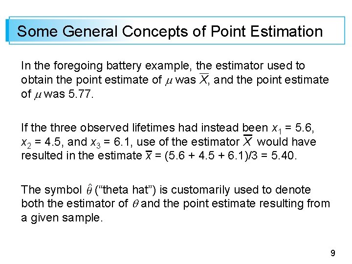
Some General Concepts of Point Estimation In the foregoing battery example, the estimator used to obtain the point estimate of was X, and the point estimate of was 5. 77. If the three observed lifetimes had instead been x 1 = 5. 6, x 2 = 4. 5, and x 3 = 6. 1, use of the estimator X would have resulted in the estimate x = (5. 6 + 4. 5 + 6. 1)/3 = 5. 40. The symbol (“theta hat”) is customarily used to denote both the estimator of and the point estimate resulting from a given sample. 9

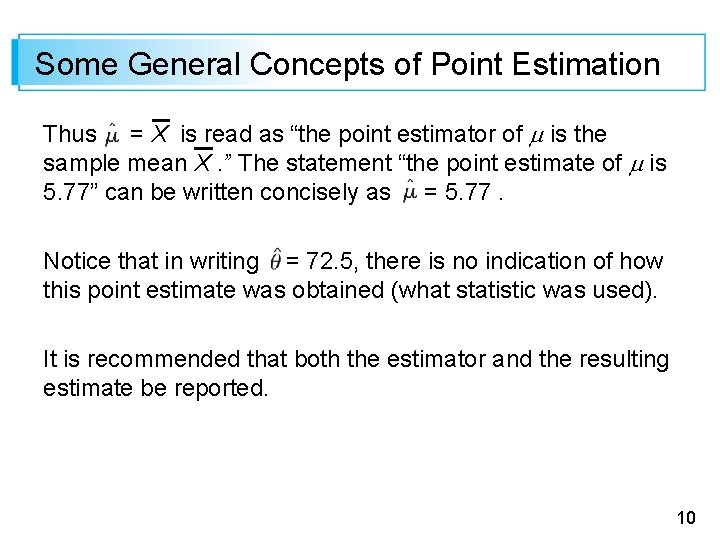
Some General Concepts of Point Estimation Thus = X is read as “the point estimator of is the sample mean X. ” The statement “the point estimate of is 5. 77” can be written concisely as = 5. 77. Notice that in writing = 72. 5, there is no indication of how this point estimate was obtained (what statistic was used). It is recommended that both the estimator and the resulting estimate be reported. 10

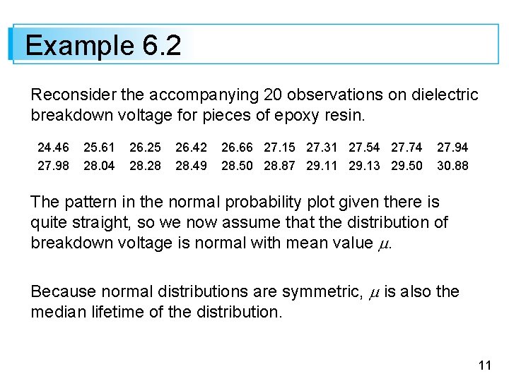
Example 6. 2 Reconsider the accompanying 20 observations on dielectric breakdown voltage for pieces of epoxy resin. 24. 46 27. 98 25. 61 28. 04 26. 25 28. 28 26. 42 28. 49 26. 66 27. 15 27. 31 27. 54 27. 74 28. 50 28. 87 29. 11 29. 13 29. 50 27. 94 30. 88 The pattern in the normal probability plot given there is quite straight, so we now assume that the distribution of breakdown voltage is normal with mean value . Because normal distributions are symmetric, is also the median lifetime of the distribution. 11

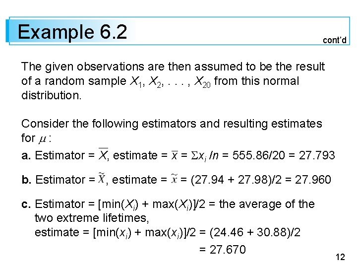
Example 6. 2 cont’d The given observations are then assumed to be the result of a random sample X 1, X 2, . . . , X 20 from this normal distribution. Consider the following estimators and resulting estimates for : a. Estimator = X, estimate = xi /n = 555. 86/20 = 27. 793 b. Estimator = , estimate = = (27. 94 + 27. 98)/2 = 27. 960 c. Estimator = [min(Xi) + max(Xi)]/2 = the average of the two extreme lifetimes, estimate = [min(xi) + max(xi)]/2 = (24. 46 + 30. 88)/2 = 27. 670 12

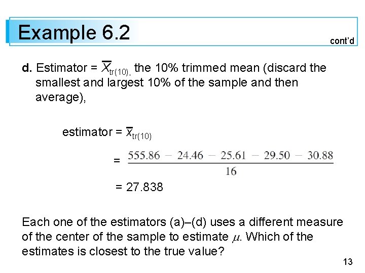
Example 6. 2 cont’d d. Estimator = Xtr(10), the 10% trimmed mean (discard the smallest and largest 10% of the sample and then average), estimator = xtr(10) = = 27. 838 Each one of the estimators (a)–(d) uses a different measure of the center of the sample to estimate . Which of the estimates is closest to the true value? 13

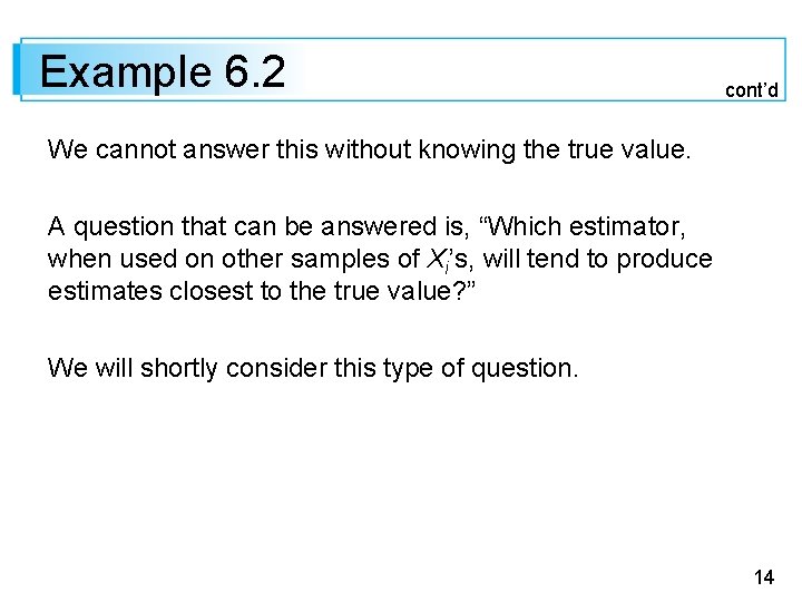
Example 6. 2 cont’d We cannot answer this without knowing the true value. A question that can be answered is, “Which estimator, when used on other samples of Xi’s, will tend to produce estimates closest to the true value? ” We will shortly consider this type of question. 14

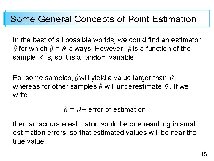
Some General Concepts of Point Estimation In the best of all possible worlds, we could find an estimator for which = always. However, is a function of the sample Xi ’s, so it is a random variable. For some samples, will yield a value larger than , whereas for other samples will underestimate . If we write = + error of estimation then an accurate estimator would be one resulting in small estimation errors, so that estimated values will be near the true value. 15

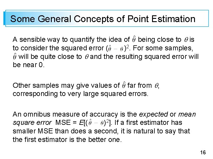
Some General Concepts of Point Estimation A sensible way to quantify the idea of being close to is to consider the squared error ( )2. For some samples, will be quite close to and the resulting squared error will be near 0. Other samples may give values of far from , corresponding to very large squared errors. An omnibus measure of accuracy is the expected or mean square error MSE = E[( )2]. If a first estimator has smaller MSE than does a second, it is natural to say that the first estimator is the better one. 16

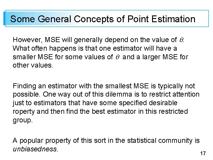
Some General Concepts of Point Estimation However, MSE will generally depend on the value of . What often happens is that one estimator will have a smaller MSE for some values of and a larger MSE for other values. Finding an estimator with the smallest MSE is typically not possible. One way out of this dilemma is to restrict attention just to estimators that have some specified desirable roperty and then find the best estimator in this restricted group. A popular property of this sort in the statistical community is unbiasedness. 17

Unbiased Estimators 18

Unbiased Estimators Suppose we have two measuring instruments; one instrument has been accurately calibrated, but the other systematically gives readings smaller than the true value being measured. When each instrument is used repeatedly on the same object, because of measurement error, the observed measurements will not be identical. However, the measurements produced by the first instrument will be distributed about the true value in such a way that on average this instrument measures what it purports to measure, so it is called an unbiased instrument. 19

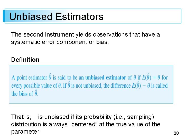
Unbiased Estimators The second instrument yields observations that have a systematic error component or bias. Definition That is, is unbiased if its probability (i. e. , sampling) distribution is always “centered” at the true value of the parameter. 20

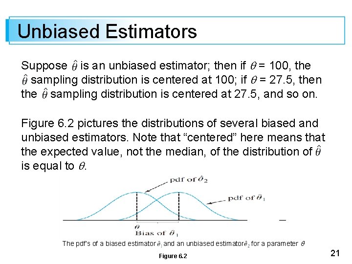
Unbiased Estimators Suppose is an unbiased estimator; then if = 100, the sampling distribution is centered at 100; if = 27. 5, then the sampling distribution is centered at 27. 5, and so on. Figure 6. 2 pictures the distributions of several biased and unbiased estimators. Note that “centered” here means that the expected value, not the median, of the distribution of is equal to . The pdf’s of a biased estimator and an unbiased estimator Figure 6. 2 for a parameter 21

Unbiased Estimators It may seem as though it is necessary to know the value of (in which case estimation is unnecessary) to see whether is unbiased. This is not usually the case, though, because unbiasedness is a general property of the estimator’s sampling distribution —where it is centered—which is typically not dependent on any particular parameter value. In Example 6. 1 the sample proportion X/n can be used as an estimator of p, where X, the number of sample successes, has a binomial distribution with parameters n and p. 22

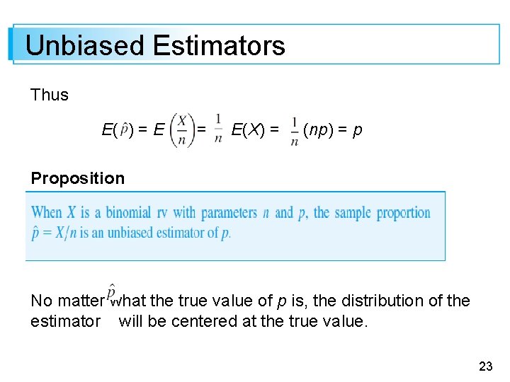
Unbiased Estimators Thus E( ) = E(X) = (np) = p Proposition No matter what the true value of p is, the distribution of the estimator will be centered at the true value. 23

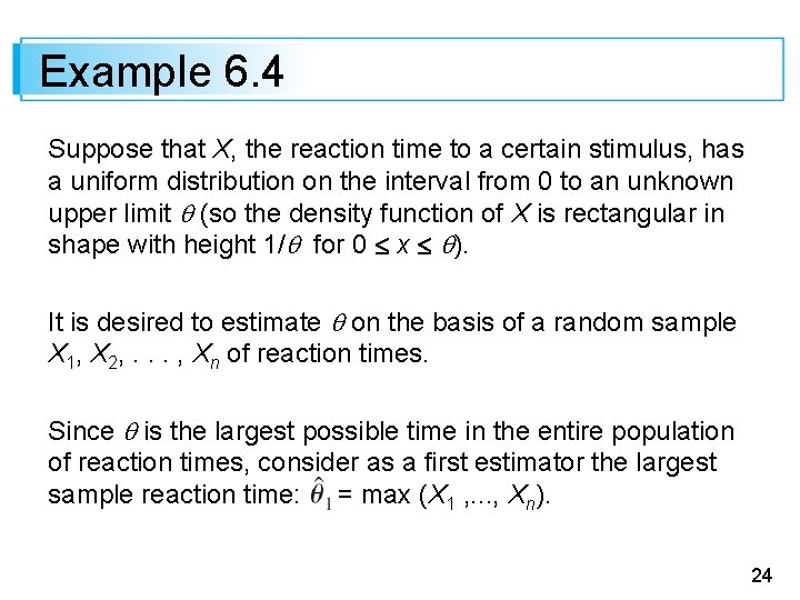
Example 6. 4 Suppose that X, the reaction time to a certain stimulus, has a uniform distribution on the interval from 0 to an unknown upper limit (so the density function of X is rectangular in shape with height 1/ for 0 x ). It is desired to estimate on the basis of a random sample X 1, X 2, . . . , Xn of reaction times. Since is the largest possible time in the entire population of reaction times, consider as a first estimator the largest sample reaction time: = max (X 1 , . . . , Xn). 24

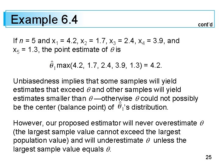
Example 6. 4 cont’d If n = 5 and x 1 = 4. 2, x 2 = 1. 7, x 3 = 2. 4, x 4 = 3. 9, and x 5 = 1. 3, the point estimate of is = max(4. 2, 1. 7, 2. 4, 3. 9, 1. 3) = 4. 2. Unbiasedness implies that some samples will yield estimates that exceed and other samples will yield estimates smaller than —otherwise could not possibly be the center (balance point) of ’s distribution. However, our proposed estimator will never overestimate (the largest sample value cannot exceed the largest population value) and will underestimate unless the largest sample value equals . 25

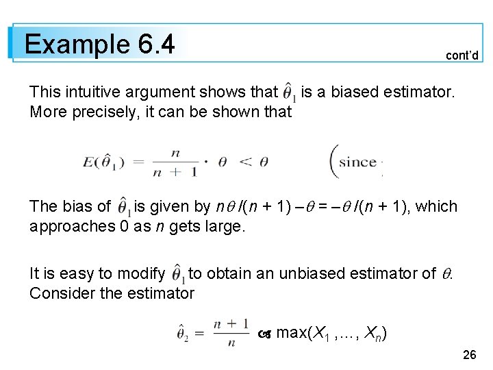
Example 6. 4 cont’d This intuitive argument shows that is a biased estimator. More precisely, it can be shown that The bias of is given by n /(n + 1) – = – /(n + 1), which approaches 0 as n gets large. It is easy to modify to obtain an unbiased estimator of . Consider the estimator max(X 1 , …, Xn) 26

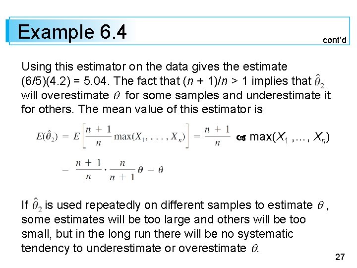
Example 6. 4 cont’d Using this estimator on the data gives the estimate (6/5)(4. 2) = 5. 04. The fact that (n + 1)/n > 1 implies that will overestimate for some samples and underestimate it for others. The mean value of this estimator is max(X 1 , …, Xn) If is used repeatedly on different samples to estimate , some estimates will be too large and others will be too small, but in the long run there will be no systematic tendency to underestimate or overestimate . 27

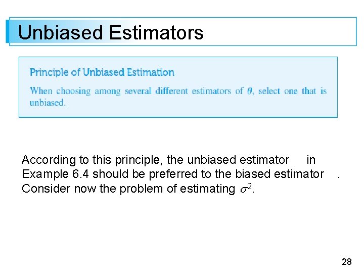
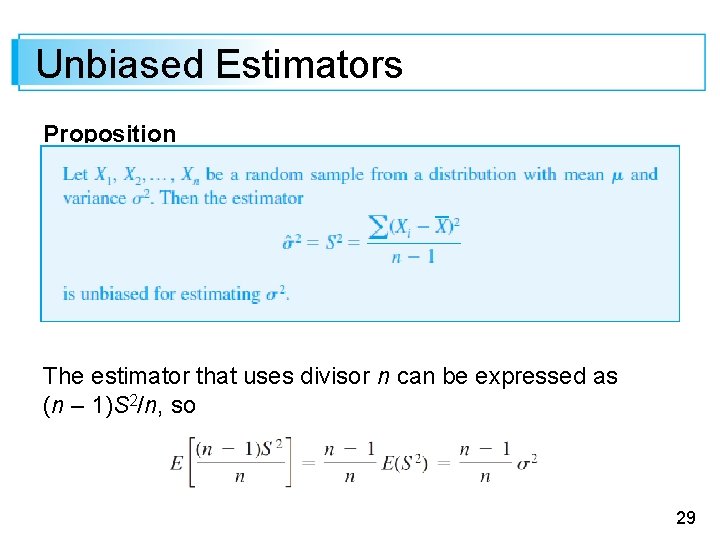
Unbiased Estimators According to this principle, the unbiased estimator in Example 6. 4 should be preferred to the biased estimator Consider now the problem of estimating 2. . 28

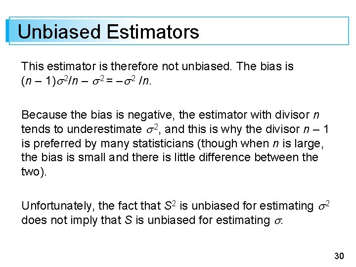
Unbiased Estimators Proposition The estimator that uses divisor n can be expressed as (n – 1)S 2/n, so 29

Unbiased Estimators This estimator is therefore not unbiased. The bias is (n – 1) 2/n – 2 = – 2 /n. Because the bias is negative, the estimator with divisor n tends to underestimate 2, and this is why the divisor n – 1 is preferred by many statisticians (though when n is large, the bias is small and there is little difference between the two). Unfortunately, the fact that S 2 is unbiased for estimating 2 does not imply that S is unbiased for estimating . 30

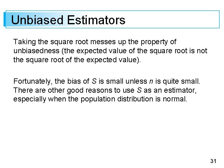
Unbiased Estimators Taking the square root messes up the property of unbiasedness (the expected value of the square root is not the square root of the expected value). Fortunately, the bias of S is small unless n is quite small. There are other good reasons to use S as an estimator, especially when the population distribution is normal. 31

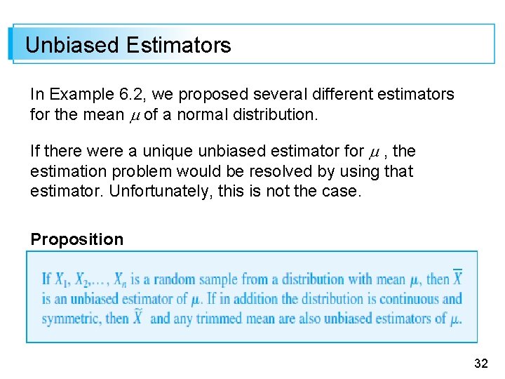
Unbiased Estimators In Example 6. 2, we proposed several different estimators for the mean of a normal distribution. If there were a unique unbiased estimator for , the estimation problem would be resolved by using that estimator. Unfortunately, this is not the case. Proposition 32

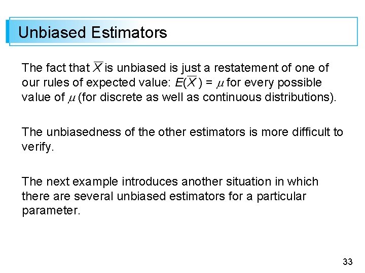
Unbiased Estimators The fact that X is unbiased is just a restatement of one of our rules of expected value: E(X ) = for every possible value of (for discrete as well as continuous distributions). The unbiasedness of the other estimators is more difficult to verify. The next example introduces another situation in which there are several unbiased estimators for a particular parameter. 33

Example 6. 5 Under certain circumstances organic contaminants adhere readily to wafer surfaces and cause deterioration in semiconductor manufacturing devices. The paper “Ceramic Chemical Filter for Removal of Organic Contaminants” (J. of the Institute of Environmental Sciences and Technology, 2003: 59– 65) discussed a recently developed alternative to conventional charcoal filters for removing organic airborne molecular contamination in cleanroom applications. 34

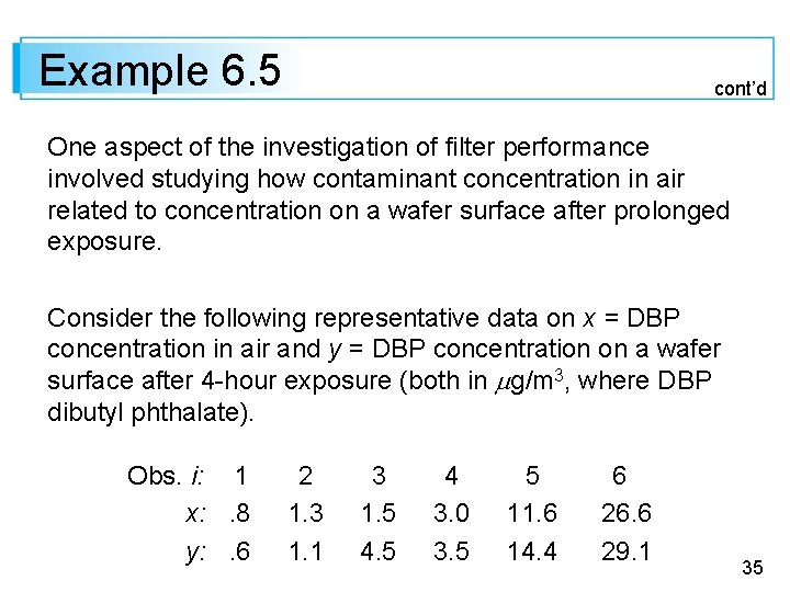
Example 6. 5 cont’d One aspect of the investigation of filter performance involved studying how contaminant concentration in air related to concentration on a wafer surface after prolonged exposure. Consider the following representative data on x = DBP concentration in air and y = DBP concentration on a wafer surface after 4 -hour exposure (both in g/m 3, where DBP dibutyl phthalate). Obs. i: 1 x: . 8 y: . 6 2 1. 3 1. 1 3 1. 5 4 3. 0 3. 5 5 11. 6 14. 4 6 26. 6 29. 1 35

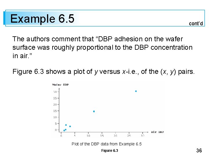
Example 6. 5 cont’d The authors comment that “DBP adhesion on the wafer surface was roughly proportional to the DBP concentration in air. ” Figure 6. 3 shows a plot of y versus x-i. e. , of the (x, y) pairs. Plot of the DBP data from Example 6. 5 Figure 6. 3 36

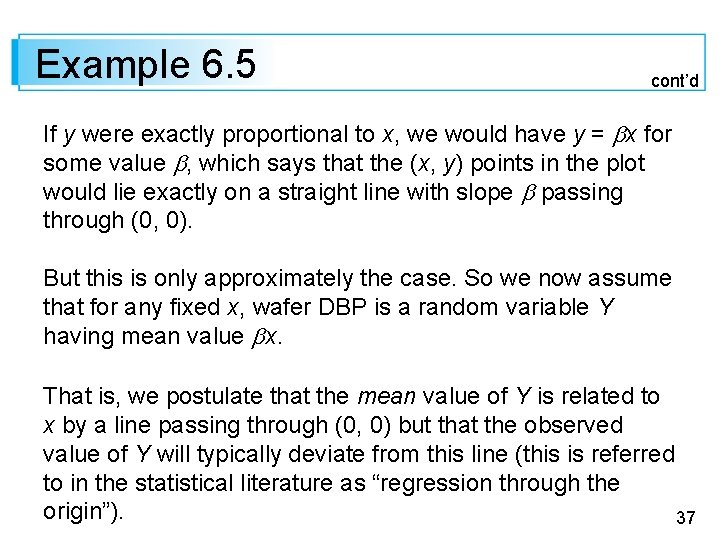
Example 6. 5 cont’d If y were exactly proportional to x, we would have y = x for some value , which says that the (x, y) points in the plot would lie exactly on a straight line with slope passing through (0, 0). But this is only approximately the case. So we now assume that for any fixed x, wafer DBP is a random variable Y having mean value x. That is, we postulate that the mean value of Y is related to x by a line passing through (0, 0) but that the observed value of Y will typically deviate from this line (this is referred to in the statistical literature as “regression through the origin”). 37

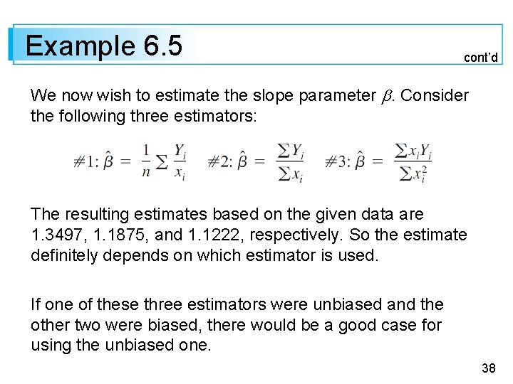
Example 6. 5 cont’d We now wish to estimate the slope parameter . Consider the following three estimators: The resulting estimates based on the given data are 1. 3497, 1. 1875, and 1. 1222, respectively. So the estimate definitely depends on which estimator is used. If one of these three estimators were unbiased and the other two were biased, there would be a good case for using the unbiased one. 38

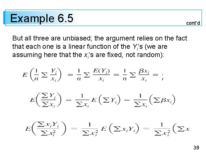
Example 6. 5 cont’d But all three are unbiased; the argument relies on the fact that each one is a linear function of the Yi’s (we are assuming here that the xi’s are fixed, not random): 39

Estimators with Minimum Variance 40

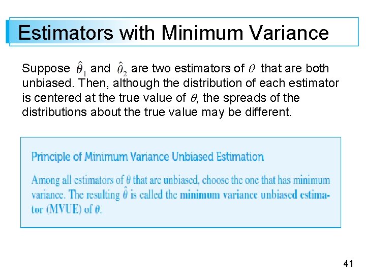
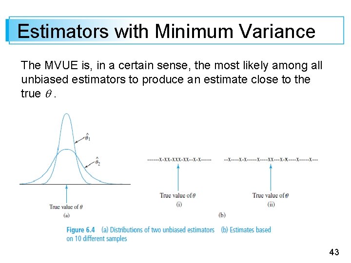
Estimators with Minimum Variance Suppose and are two estimators of that are both unbiased. Then, although the distribution of each estimator is centered at the true value of , the spreads of the distributions about the true value may be different. 41

Estimators with Minimum Variance 42

Estimators with Minimum Variance The MVUE is, in a certain sense, the most likely among all unbiased estimators to produce an estimate close to the true . 43

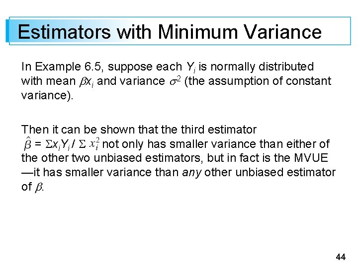
Estimators with Minimum Variance In Example 6. 5, suppose each Yi is normally distributed with mean xi and variance 2 (the assumption of constant variance). Then it can be shown that the third estimator = xi. Yi / not only has smaller variance than either of the other two unbiased estimators, but in fact is the MVUE —it has smaller variance than any other unbiased estimator of . 44

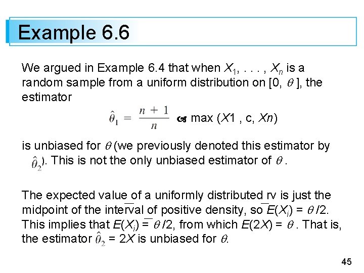
Example 6. 6 We argued in Example 6. 4 that when X 1, . . . , Xn is a random sample from a uniform distribution on [0, ], the estimator max (X 1 , c, Xn) is unbiased for (we previously denoted this estimator by ). This is not the only unbiased estimator of . The expected value of a uniformly distributed rv is just the midpoint of the interval of positive density, so E(Xi) = /2. This implies that E(Xi) = /2, from which E(2 X) = . That is, the estimator = 2 X is unbiased for . 45

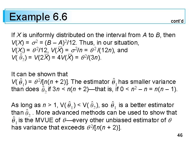
Example 6. 6 cont’d If X is uniformly distributed on the interval from A to B, then V(X) = 2 = (B – A)2/12. Thus, in our situation, V(Xi) = 2/12, V(X) = 2/n = 2 /(12 n), and V( ) = V(2 X) = 4 V(X) = 2/(3 n). It can be shown that V( ) = 2/[n(n + 2)]. The estimator has smaller variance than does if 3 n < n(n + 2)—that is, if 0 < n 2 – n = n(n – 1). As long as n > 1, V( ) < V( ), so is a better estimator than. More advanced methods can be used to show that is the MVUE of —every other unbiased estimator of has variance that exceeds 2/[n(n + 2)]. 46

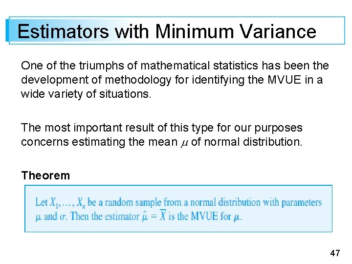
Estimators with Minimum Variance One of the triumphs of mathematical statistics has been the development of methodology for identifying the MVUE in a wide variety of situations. The most important result of this type for our purposes concerns estimating the mean of normal distribution. Theorem 47

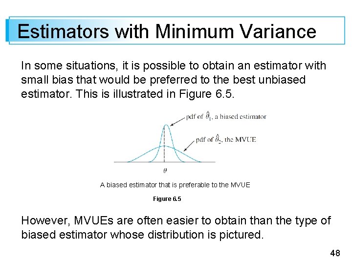
Estimators with Minimum Variance In some situations, it is possible to obtain an estimator with small bias that would be preferred to the best unbiased estimator. This is illustrated in Figure 6. 5. A biased estimator that is preferable to the MVUE Figure 6. 5 However, MVUEs are often easier to obtain than the type of biased estimator whose distribution is pictured. 48

Some Complications 49

Some Complications The last theorem does not say that in estimating a population mean , the estimator X should be used irrespective of the distribution being sampled. 50

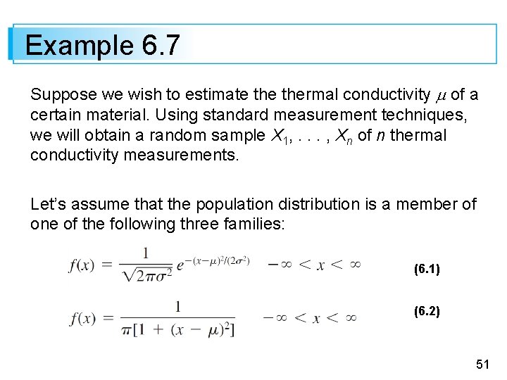
Example 6. 7 Suppose we wish to estimate thermal conductivity of a certain material. Using standard measurement techniques, we will obtain a random sample X 1, . . . , Xn of n thermal conductivity measurements. Let’s assume that the population distribution is a member of one of the following three families: (6. 1) (6. 2) 51

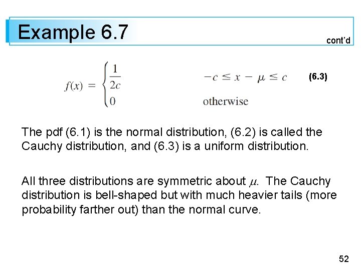
Example 6. 7 cont’d (6. 3) The pdf (6. 1) is the normal distribution, (6. 2) is called the Cauchy distribution, and (6. 3) is a uniform distribution. All three distributions are symmetric about . The Cauchy distribution is bell-shaped but with much heavier tails (more probability farther out) than the normal curve. 52

Example 6. 7 cont’d The uniform distribution has no tails. The four estimators for m considered earlier are X , , Xe (the average of the two extreme observations), and Xtr(10), a trimmed mean. The very important moral here is that the best estimator for depends crucially on which distribution is being sampled. In particular, 1. If the random sample comes from a normal distribution, then X is the best of the four estimators, since it has minimum variance among all unbiased estimators. 53

Example 6. 7 cont’d 2. If the random sample comes from a Cauchy distribution, then X and Xe are terrible estimators for , whereas is quite good (the MVUE is not known); X is bad because it is very sensitive to outlying observations, and the heavy tails of the Cauchy distribution make a few such observations likely to appear in any sample. 3. If the underlying distribution is uniform, the best estimator is Xe; this estimator is greatly influenced by outlying observations, but the lack of tails makes such observations impossible. 54

Example 6. 7 cont’d 4. The trimmed mean is best in none of these three situations but works reasonably well in all three. That is, Xtr(10), does not suffer too much in comparison with the best procedure in any of the three situations. 55

Reporting a Point Estimate: The Standard Error 56

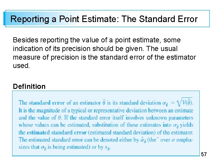
Reporting a Point Estimate: The Standard Error Besides reporting the value of a point estimate, some indication of its precision should be given. The usual measure of precision is the standard error of the estimator used. Definition 57

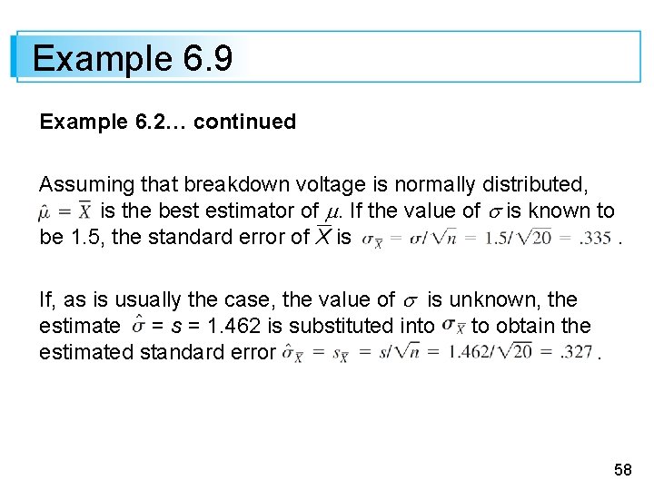
Example 6. 9 Example 6. 2… continued Assuming that breakdown voltage is normally distributed, is the best estimator of . If the value of is known to be 1. 5, the standard error of X is. If, as is usually the case, the value of is unknown, the estimate = s = 1. 462 is substituted into to obtain the estimated standard error. 58

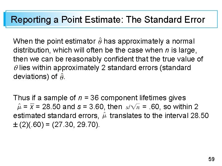
Reporting a Point Estimate: The Standard Error When the point estimator has approximately a normal distribution, which will often be the case when n is large, then we can be reasonably confident that the true value of lies within approximately 2 standard errors (standard deviations) of. Thus if a sample of n = 36 component lifetimes gives = x = 28. 50 and s = 3. 60, then =. 60, so within 2 estimated standard errors, translates to the interval 28. 50 (2)(. 60) = (27. 30, 29. 70). 59

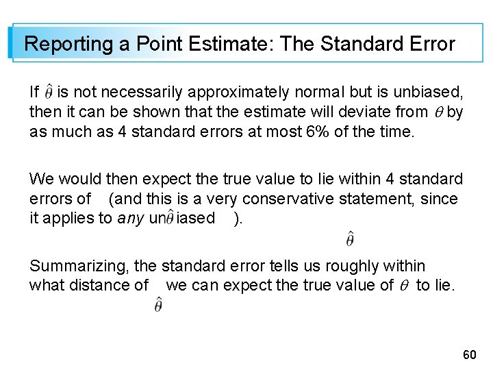
Reporting a Point Estimate: The Standard Error If is not necessarily approximately normal but is unbiased, then it can be shown that the estimate will deviate from by as much as 4 standard errors at most 6% of the time. We would then expect the true value to lie within 4 standard errors of (and this is a very conservative statement, since it applies to any unbiased ). Summarizing, the standard error tells us roughly within what distance of we can expect the true value of to lie. 60

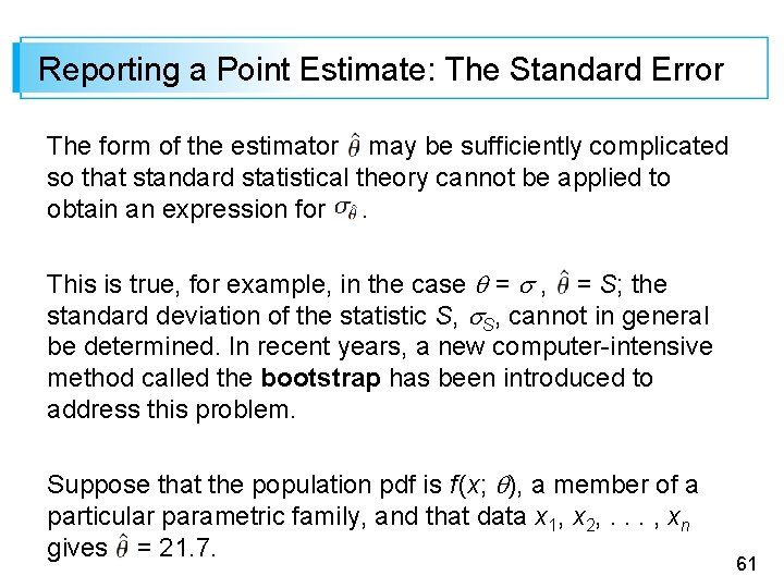
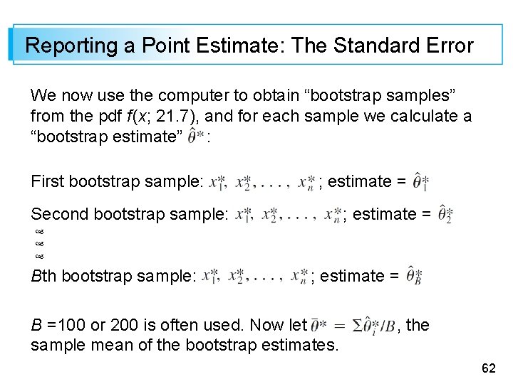
Reporting a Point Estimate: The Standard Error The form of the estimator may be sufficiently complicated so that standard statistical theory cannot be applied to obtain an expression for. This is true, for example, in the case = , = S; the standard deviation of the statistic S, cannot in general be determined. In recent years, a new computer-intensive method called the bootstrap has been introduced to address this problem. Suppose that the population pdf is f (x; ), a member of a particular parametric family, and that data x 1, x 2, . . . , xn gives = 21. 7. 61

Reporting a Point Estimate: The Standard Error We now use the computer to obtain “bootstrap samples” from the pdf f (x; 21. 7), and for each sample we calculate a “bootstrap estimate” : First bootstrap sample: ; estimate = Second bootstrap sample: ; estimate = Bth bootstrap sample: ; estimate = B =100 or 200 is often used. Now let sample mean of the bootstrap estimates. , the 62

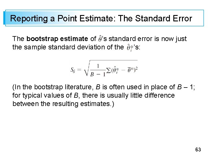
Reporting a Point Estimate: The Standard Error The bootstrap estimate of ’s standard error is now just the sample standard deviation of the ’s: (In the bootstrap literature, B is often used in place of B – 1; for typical values of B, there is usually little difference between the resulting estimates. ) 63

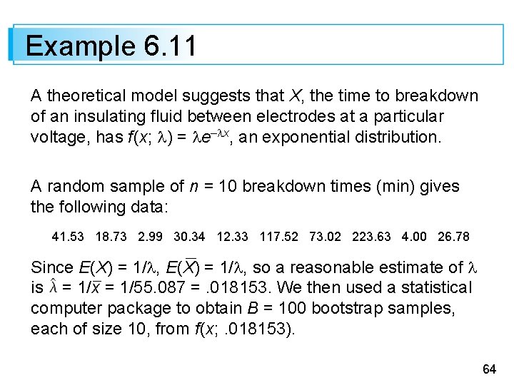
Example 6. 11 A theoretical model suggests that X, the time to breakdown of an insulating fluid between electrodes at a particular voltage, has f (x; ) = e– x, an exponential distribution. A random sample of n = 10 breakdown times (min) gives the following data: 41. 53 18. 73 2. 99 30. 34 12. 33 117. 52 73. 02 223. 63 4. 00 26. 78 Since E(X) = 1/ , so a reasonable estimate of is = 1/x = 1/55. 087 =. 018153. We then used a statistical computer package to obtain B = 100 bootstrap samples, each of size 10, from f (x; . 018153). 64

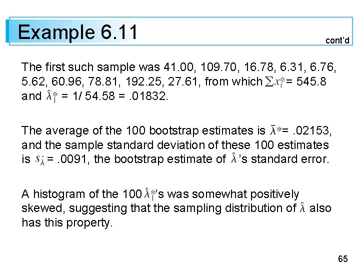
Example 6. 11 cont’d The first such sample was 41. 00, 109. 70, 16. 78, 6. 31, 6. 76, 5. 62, 60. 96, 78. 81, 192. 25, 27. 61, from which = 545. 8 and = 1/ 54. 58 =. 01832. The average of the 100 bootstrap estimates is =. 02153, and the sample standard deviation of these 100 estimates is =. 0091, the bootstrap estimate of ’s standard error. A histogram of the 100 ’s was somewhat positively skewed, suggesting that the sampling distribution of also has this property. 65