1 JianJiun Ding National Taiwan University 723 531

1 丁建均 (Jian-Jiun Ding) National Taiwan University 辦公室：明達館 723室， 實驗室：明達館 531室 聯絡電話： (02)33669652 Major：Digital Signal Processing Digital Image Processing

Research Fields [A. Time-Frequency Analysis] (1) Time-Frequency Analysis (page 4) (2) Music Signal Analysis (page 17) : main topics that I researched in recent years (3) Fractional Fourier Transform (page 20) (4) Wavelet Transform (page 34) [B. Image Processing] (5) Image Compression (page 37) (6) Edge and Corner Detection (page 45) (7) Segmentation (page 49) 2 (8) Pattern Recognition (Face, Character) (page 54)

3 [C. Fast Algorithms] (9) Fast Algorithms (10) Integer Transforms (page 56) (11) Number Theory, Haar Transform, Walsh Transform [D. Applications of Signal Processing] (12) Optical Signal Processing (page 62) (13) Acoustics (14) Bioinformatics (page 64) [E. Theories for Signal Processing] (15) Quaternions (page 68) (16) Eigenfunctions, Eigenvectors, and Prolate Spheroidal Wave Function (17) Signal Analysis (Cepstrum, Hilbert, CDMA)

1. Time-Frequency Analysis http: //djj. ee. ntu. edu. tw/TFW. htm Fourier transform (FT) Time-Domain Frequency Domain Some things make the FT not practical: (1) Only the case where t 0 t t 1 is interested. (2) Not all the signals are suitable for analyzing in the frequency domain. It is hard to analyze the signal whose instantaneous frequency varies with time. 4

Example: x(t) = cos( t) when t < 10, x(t) = cos(3 t) when 10 t < 20, x(t) = cos(2 t) when t 20 (FM signal) 5

6 Using Time-Frequency analysis x(t) = cos( t) when t < 10, x(t) = cos(2 t) when t 20 x(t) = cos(3 t) when 10 t < 20, (FM signal) f -axis t -axis Left：using Gray level to represent the amplitude of X(t, f) Right：slicing along t = 15 t -axis

7 Several Time-Frequency Distribution Short-Time Fourier Transform (STFT) with Rectangular Mask Gabor Transform avoid cross-term less clarity Wigner Distribution Function with cross-term high clarity Gabor-Wigner Transform (Proposed) avoid cross-term high clarity

8 Cohen’s Class Distribution where S Transform Hilbert-Huang Transform

Instantaneous Frequency 瞬時頻率 9 If then the instantaneous frequency of x(t) are 自然界瞬時頻率會隨時間而改變的例子 音樂，語音信號, Doppler effect, seismic waves, optics, radar system, rectangular function, …………… In fact, in addition to sinusoid-like functions, the instantaneous frequencies of other functions will inevitably vary with time.

Applications of Time-Frequency Analysis (1) Finding Instantaneous Frequency (2) Music Signal Analysis (3) Sampling Theory (4) Modulation and Multiplexing (5) Filter Design (6) Random Process Analysis (7) Signal Decomposition (8) Electromagnetic Wave Propagation (9) Optics (10) Radar System Analysis (11) Signal Identification (12) Acoustics (13) Biomedical Engineering (14) Spread Spectrum Analysis (15) System Modeling (16) Image Processing (17) Economic Data Analysis (18) Signal Representation (19) Data Compression (20) Seismology (21) Geology 10

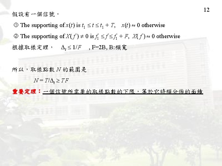
11 Conventional Sampling Theory Nyquist Criterion New Sampling Theory (1) t can vary with time (2) Number of sampling points == Area of time frequency distribution

13 Modulation and Multiplexing spectrum of signal 1 -B 1 spectrum of signal 2 -B 2 not overlapped B 2

14 Improvement of Time-Frequency Analysis (1) Computation Time (2) Tradeoff of the cross term problem and clarification

left: x 1(t) = 1 for |t| 6, x 1(t) = 0 otherwise, -axis Gabor t -axis WDF t -axis right: x 2(t) = cos(6 t 0. 05 t 2) 15

16 Gabor-Wigner Transform -axis avoiding the cross-term problem and high clarity t -axis

17 2. Music Signal Analysis Using the time-frequency analysis 聲音檔：http: //djj. ee. ntu. edu. tw/Chord. wav So Mi Do La Fa Re

聲音檔：http: //djj. ee. ntu. edu. tw/air. mp 3 time-frequency analysis 18

20 3. Fractional Fourier Transform Performing the Fourier transform a times (a can be non-integer) Fourier Transform (FT) generalization Fractional Fourier Transform (FRFT) , When = 0. 5 , the FRFT becomes the FT. = a/2

21 Fractional Fourier Transform (FRFT) , When = 0: = a/2. (identity) When = 0. 5 : When is not equal to a multiple of 0. 5 , the FRFT is equivalent to doing /(0. 5 ) times of the Fourier transform. when = 0. 1 doing the FT 0. 2 times; when = 0. 25 doing the FT 0. 5 times; when = /6 doing the FT 1/3 times;

22 Physical Meaning: Transform a Signal into the Fractional domain, which is the intermediate of the time domain and the frequency domain.

Time domain Frequency domain fractional domain Modulation Shifting Modulation + Shifting Differentiation −j 2 f Differentiation and j 2 f Differentiation and −j 2 f is some constant phase 23

Why do we use the fractional Fourier transform? To solve the problems that cannot be solved by the Fourier transform Example: Filter Design Conventional filter design: x(t): input x(t) = s(t) (signal) + n(t) (noise) y(t): output (We want that y(t) s(t)) H( ): the transfer function of the filter. Filter design by the fractional Fourier transform (FRFT): (replace the FT and the IFT by the FRFTs with parameters and ) 24

When x(t) = triangular signal + chirp noise exp[j 0. 25(t 4. 12)2] 25

26 The Fourier transform is suitable to filter out the noise that is a combination of sinusoid functions exp(j 0 t). The fractional Fourier transform (FRFT) is suitable to filter out the noise that is a combination of higher order exponential functions exp[j(nk tk + nk-1 tk-1 + nk-2 tk-2 + ……. + n 2 t 2 + n 1 t)] For example: chirp function exp(jn 2 t 2) With the FRFT, many noises that cannot be removed by the FT will be filtered out successfully.

From the view points of Time-Frequency Analysis: 27 [Theorem] The FRFT with parameter is equivalent to the clockwise rotation operation with angle for Wigner distribution functions (or for Gabor transforms) FRFT = with angle The Gabor Transform for the FRFT of the rectangular function. = 0 (identity), /6 2 /6 /2 (FT) 4 /6 5 /6 horizon: t-axis, vertical: f-axis [Ref 1] S. C. Pei and J. J. Ding, “Relations between Gabor transforms and fractional Fourier transforms and their applications for signal processing, ” IEEE Trans. Signal Processing, vol. 55, no. 10, pp. 4839 -4850, Oct. 2007.

28 Filter designed by the fractional Fourier transform 比較：Filter Designed by the Fourier transform f-axis Signal noise FRFT noise Signal FRFT t-axis cutoff line

以時頻分析的觀點，傳統濾波器是垂直於 f-axis 做切割的 f-axis stop band f 0 cutoff line pass band t-axis 而用 fractional Fourier transform 設計的濾波器是，是由斜的方向作切割 f-axis cutoff line 和 f-axis 在逆時針方向的夾 角為 stop band u 0 pass band cutoff line 29

Gabor Transform for signal + 0. 3 exp[j 0. 06(t 1)3 j 7 t] 30 fractional axis t-axis Advantage: Easy to estimate the character of a signal in the fractional domain Proposed an efficient way to find the optimal parameter

31 In fact, all the applications of the Fourier transform (FT) are also the applications of the fractional Fourier transform (FRFT), and using the FRFT instead of the FT for these applications may improve the performance. Filter Design : developed by us improved the previous works Signal synthesis (compression, random process, fractional wavelet transform) Correlation (space variant pattern recognition) Communication (modulation, multiplexing, multiple-path problem) Sampling Solving differential equation Image processing (asymmetry edge detection, directional corner detection) Optical system analysis (system model, self-imaging phenomena) Wave propagation analysis (radar system, GRIN-medium system)

Invention: 32 [Ref 2] N. Wiener, “Hermitian polynomials and Fourier analysis, ” Journal of Mathematics Physics MIT, vol. 18, pp. 70 -73, 1929. Re-invention [Ref 3] V. Namias, “The fractional order Fourier transform and its application to quantum mechanics, ” J. Inst. Maths. Applics. , vol. 25, pp. 241265, 1980. Introduction for signal processing [Ref 4] L. B. Almeida, “The fractional Fourier transform and time-frequency representations, ” IEEE Trans. Signal Processing, vol. 42, no. 11, pp. 30843091, Nov. 1994. Recent development Pei, Ding (after 1995), Ozaktas, Mendlovic, Kutay, Zalevsky, etc.

My works related to the fractional Fourier transform (FRFT) Extensions: Discrete fractional Fourier transform Fractional cosine, and Hartley transform, Two-dimensional form, N-D form, Simplified fractional Fourier transform Fractional Hilbert transform, Foundation theory: relations between the FRFT and the wellknown time-frequency analysis tools (e. g. , the Wigner distribution function and the Gabor transform) Applications: sampling, encryption, corner and edge detection, self -imaging phenomena, bandwidth saving, multiple-path problem analysis, random process analysis, filter design Solving the problem for implementation 33

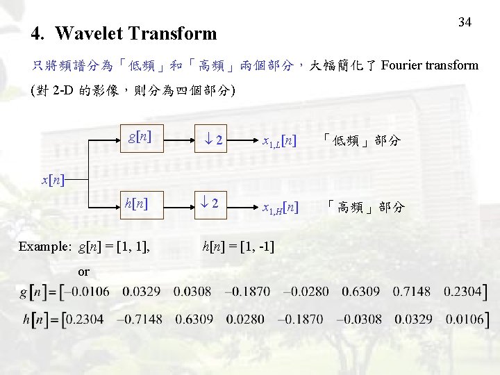
35 The result of the wavelet transform for a 2 -D image lowpass for x lowpass for y highpass for x lowpass for y highpass for y

36 Applications for Wavelets -- JPEG 2000 (image compression) -- filter design -- edge and corner detection -- pattern recognition -- biomedical engineering

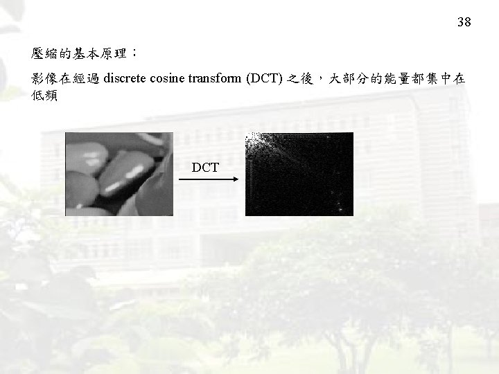
37 5. Image Compression Conventional JPEG method: Separate the original image into many 8*8 blocks, then using the DCT to code each blocks. DCT: discrete cosine transform PS: 感謝 2008年畢業的黃俊德同學

39 JPEG 是當前最普及的影像壓縮格式。 問題：壓縮率高的時候，會產生 blocking effect Compression ratio = 53. 4333 RMSE = 10. 9662

New Method: Edge-Based Segmentation and Compression 和小時候畫圖的方法類似 40

41 • Segmentation-based image compression Boundary An image Boundary Compression Image Segmentation Image Segment Bit stream Image Segment Compression

42 Original Image An 100 x 100 image By JPEG Bytes: 1295, RMSE: 2. 39 By Proposed Method Bytes: 456, RMSE: 2. 54

43 原圖 (10000 bytes) 使用 JPEG (233 bytes) 使用 JPEG (692 bytes) 使用新方法 (165 bytes)

6. Edge and Corner Detection Why should we perform edge and corner detection? --Segmentation --Compression 45

46 Simplest way for edge detection: differentiation

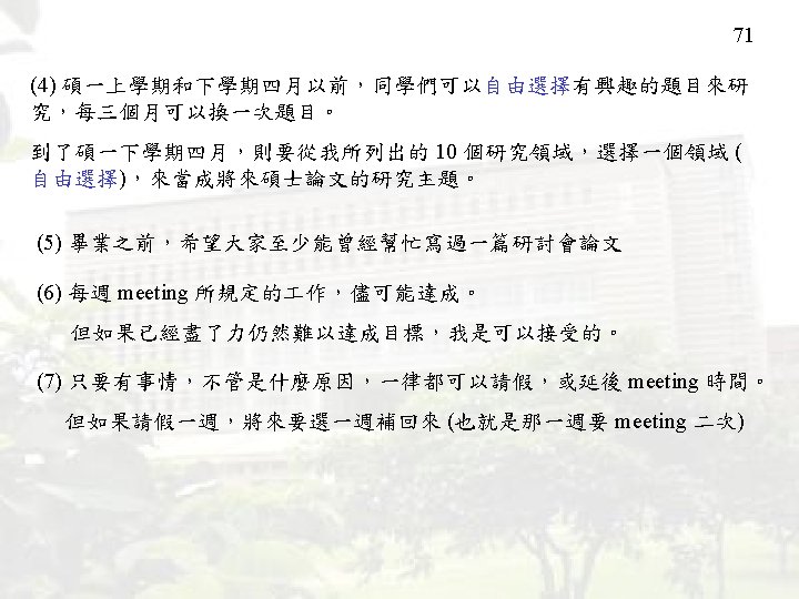
47 Doing difference x[n] x[n 1] = x[n] (convolution) with h[n] = 1 for n = 0, h[n] = -1 for n = 1, h[n] = 0 otherwise. Other ways for edge detection: convolution with a longer odd function x[n]

48 Corner Detection by Harris’ algorithm by proposed algorithm

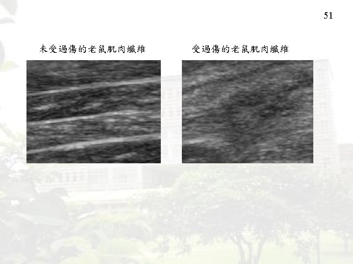
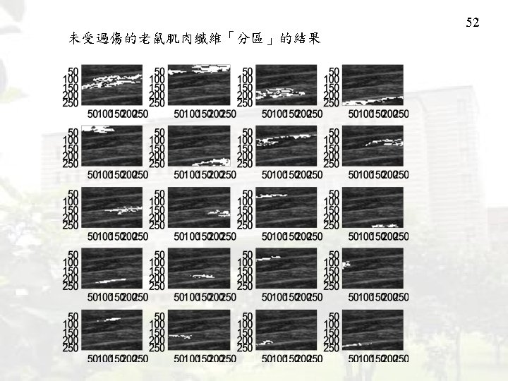
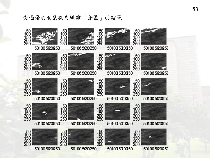
7. Segmentation Important for compression biomedical engineering object identification 49

50 Conventional method: 97. 87 sec New method: 1. 02 sec

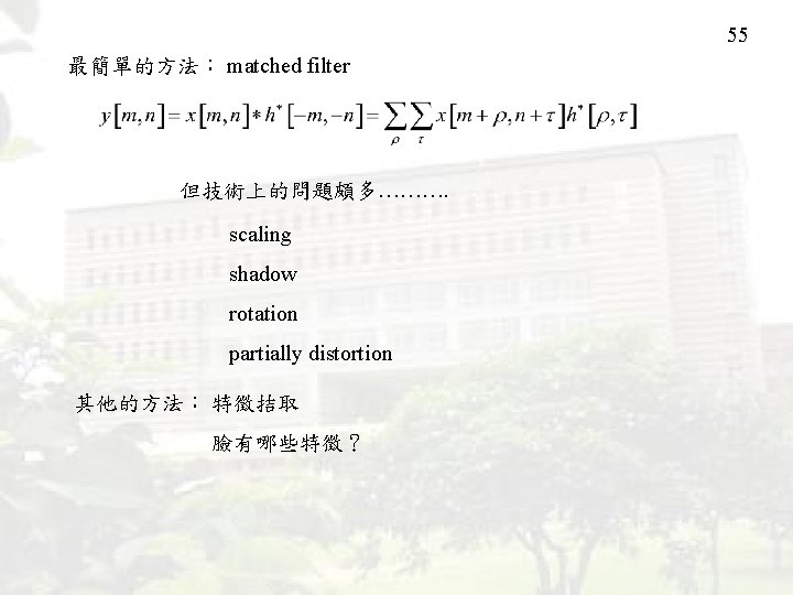
8. Pattern Recognition including face recognition character recognition 應用很廣： security, identification, computer vision ………… 54

56 10. Integer Transform Conversion Integer Transform: The discrete linear operation whose entries are summations of 2 k. , ak = 0 or 1 or , C is an integer.

57 Problem: Most of the discrete transforms are non-integer ones. DFT, DCT, Karhunen-Loeve transform, RGB to YIQ color transform --- To implement them exactly, we should use floating-point processor --- To implement them by fixed-point processor, we should approximate it by an integer transform. However, after approximation, the reversibility property is always lost.

Integer RGB to YCb. Cr Transform This is used in JPEG 2000. 58

59 [Integer Transform Conversion]: Converting all the non-integer transform into an integer transform that achieve the following 6 Goals: A, A-1: original non-integer transform pair, (Goal 1) Integerization (Goal 2) Reversibility , B, B : integer transform pair , bk and b k are integers. . (Goal 3) Bit Constraint The denominator 2 k should not be too large. (Goal 4) Accuracy B A, (Goal 5): Less Complexity (Goal 6) Easy to Design B A-1 (or B A, B -1 A-1)

60 Development of Integer Transforms: (A) Prototype Matrix Method (Partially my work) (suitable for 2, 4, 8 and 16 -point DCT, DST, DFT) (B) Lifting Scheme (suitable for 2 k-point DCT, DST, DFT) (C) Triangular Matrix Scheme (suitable for any matrices, satisfies Goals 1 and 2) (D) Improved Triangular Matrix Scheme (My works) (suitable for any matrices, satisfies Goals 1 ~ 6)

61 References Related to the Integer Transform [Ref. 1] W. K. Cham, “Development of integer cosine transform by the principles of dynamic symmetry, ” Proc. Inst. Elect. Eng. , pt. 1, vol. 136, no. 4, pp. 276 -282, Aug. 1989. [Ref. 2] S. C. Pei and J. J. Ding, “The integer Transforms analogous to discrete trigonometric transforms, ” IEEE Trans. Signal Processing, vol. 48, no. 12, pp. 3345 -3364, Dec. 2000. [Ref. 3] T. D. Tran, “The bin. DCT: fast multiplierless approximation of the DCT, ” IEEE Signal Proc. Lett. , vol. 7, no. 6, pp. 141 -144, June 2000. [Ref. 4] P. Hao and Q. Shi. , “Matrix factorizations for reversible integer mapping, ” IEEE Trans. Signal Processing, vol. 49, no. 10, pp. 23142324, Oct. 2001. [Ref. 5] S. C. Pei and J. J. Ding, “Reversible Integer Color Transform with Bit-Constraint, ” accepted by ICIP 2005. [Ref. 6] S. C. Pei and J. J. Ding, “Improved Integer Color Transform, ” in preparation

62 12. Optical Signal Processing and Fractional Fourier Transform lens, (focal length = f) free space, (length = z 1) free space, (length = z 2) f = z 1 = z 2 Fourier Transform f z 1, z 2 but z 1 = z 2 Fractional Fourier Transform (see page 20) f z 1 z 2 Fractional Fourier Transform multiplied by a chirp

64 14. Discrete Correlation Algorithm for DNA Sequence Comparison [Reference] S. C. Pei, J. J. Ding, and K. H. Hsu, “DNA sequence comparison and alignment by the discrete correlation algorithm, ” submitted. There are four types of nucleotide in a DNA sequence: adenine (A), guanine (G), thymine (T), cytosine (C) Unitary Mapping bx[ ] = 1 bx[ ] = j if x[ ] = ‘A’, if x[ ] = ‘G’, bx[ ] = 1 bx[ ] = j if x[ ] = ‘T’, if x[ ] = ‘C’. y = ‘AACTGAA’, by = [1, 1, j, 1, j, 1, 1].

65 Discrete Correlation Algorithm for DNA Sequence Comparison For two DNA sequences x and y, if where Then there are s[n] nucleotides of x[n+ ] that satisfies x[n+ ] = y[ ]. Example: x = ‘GTAGCTGAAC’, y = ‘AACTGAA’, . x= ‘GTAGCTGAAC’, y (shifted 7 entries rightward) = ‘AACTGAA’.

66 Example: x = ‘GTAGCTGAAC’, y = ‘AACTGAA’, s[n] = . Checking: x= y= ‘GTAGCTGAAC’, ‘AACTGAA’. (no entry match) x= ‘GTAGCTGAAC’, y = (shifted 2 entries rightward) ‘AACTGAA’. (6 entries match) x= ‘GTAGCTGAAC’, y (shifted 7 entries rightward) = ‘AACTGAA’. (7 entries match)

67 Advantage of the Discrete Correlation Algorithm: ---The complexity of the conventional sequence alignments is O(N 2) ---For the discrete correlation algorithm, the complexity is reduced to O(N log 2 N) or O(N log 2 N + b 2) b: the length of the matched subsequences Experiment: Local alignment for two 3000 -entry DNA sequences Using conventional dynamic programming Computation time: 87 sec. Using the proposed discrete correlation algorithm: Computation time: 4. 13 sec.

68 15. Quaternion 翻譯成“四元素”，Generalization of complex number Complex number: a + ib i 2 = 1 real part imaginary part Quaternion: a + ib + jc + kd real part i 2 = j 2 = k 2 = 1 3 imaginary parts [Ref 18] S. C. Pei, J. J. Ding, and J. H. Chang, “Efficient implementation of quaternion Fourier transform, ” IEEE Trans. Signal Processing, vol. 49, no. 11, pp. 2783 -2797, Nov. 2001. [Ref 19] S. C. Pei, J. H. Chang, and J. J. Ding, “Commutative reduced biquaternions for signal and image processing, ” IEEE Trans. Signal Processing, vol. 52, pp. 2012 -2031, July 2004.

Application of quaternion a + ib + jc + kd: --Color image processing a + i. R + j. G + k. B represent an RGB image --Multiple-Channel Analysis 4 real channels or 2 complex channels a b c d = a+jb c+jd 69