Quantitative Earthquake Prediction twenty years of realtime application

Quantitative Earthquake Prediction: twenty years of real-time application and testing Vladimir G. Kossobokov International Institute of Earthquake Prediction Theory and Mathematical Geophysics, Russian Academy of Sciences, 79 -2 Warshavskoye Shosse, Moscow 113556, Russian Federation Institut de Physique du Globe de Paris, 4 Place Jussieu, 75252 Paris, Cedex 05, France E-mail: volodya@mitp. ru or volodya@ipgp. jussieu. fr

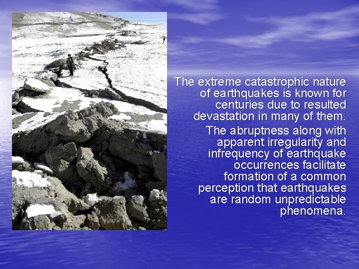
The extreme catastrophic nature of earthquakes is known for centuries due to resulted devastation in many of them. The abruptness along with apparent irregularity and infrequency of earthquake occurrences facilitate formation of a common perception that earthquakes are random unpredictable phenomena.

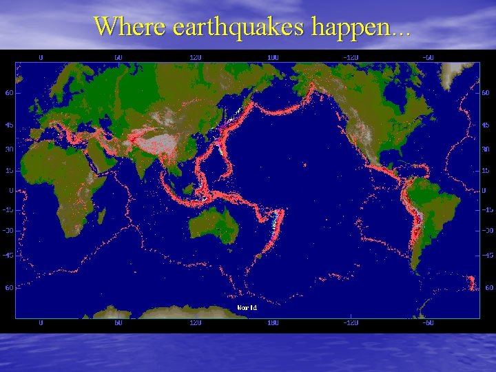
Where earthquakes happen. . .

How often. . . Global Number of Earthquakes vs. Time Global Hypocenters Data Base CD‑ROM, 1989. NEIC/USGS, Denver, CO. and its PDE and QED updates to the present

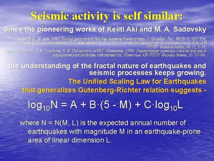
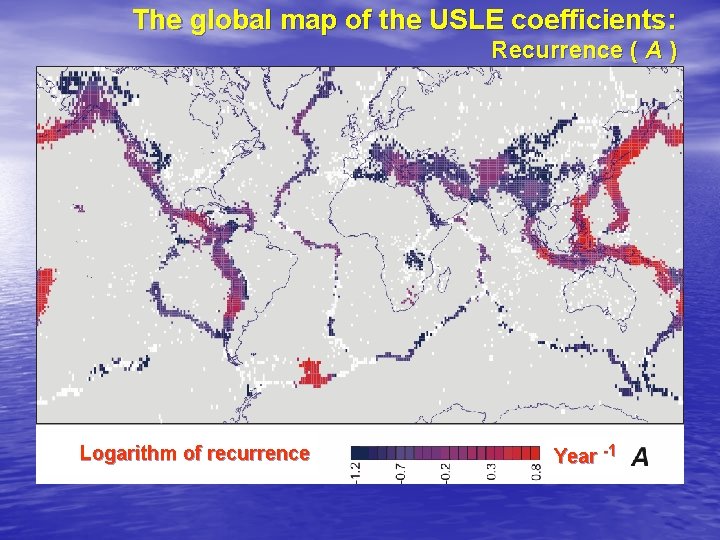
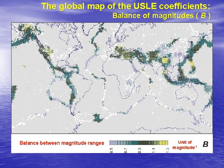
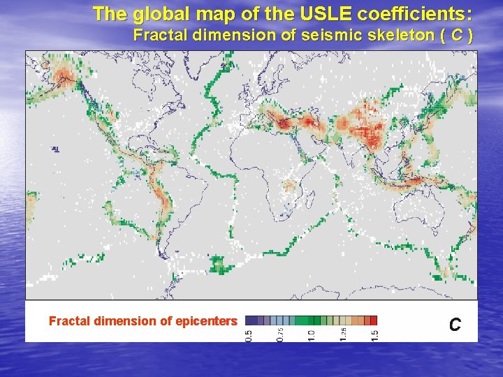
Seismic activity is self similar: Since the pioneering works of Keiiti Aki and M. A. Sadovsky Okubo, P. G. , K. Aki, 1987. Fractal geometry in the San Andreas Fault system. J. Geophys. Res. , 92 (B 1), 345 -356; Садовский М. А. , Болховитинов Л. Г. , Писаренко В. Ф. , 1982. О свойстве дискретности горных пород. Изв. АН СССР. Физика Земли, № 12, 3 -18; Садовский, М. А. , Т. В. Голубева, В. Ф. Писаренко, и М. Г. Шнирман, 1984. Характерные размеры горной породы и иерархические свойства сейсмичности. Известия АН СССР. Физика Земли, 20: 87– 96. the understanding of the fractal nature of earthquakes and seismic processes keeps growing. The Unified Scaling Law for Earthquakes that generalizes Gutenberg-Richter relation suggests - log 10 N = A + B·(5 - M) + C·log 10 L where N = N(M, L) is the expected annual number of earthquakes with magnitude M in an earthquake-prone area of linear dimension L.

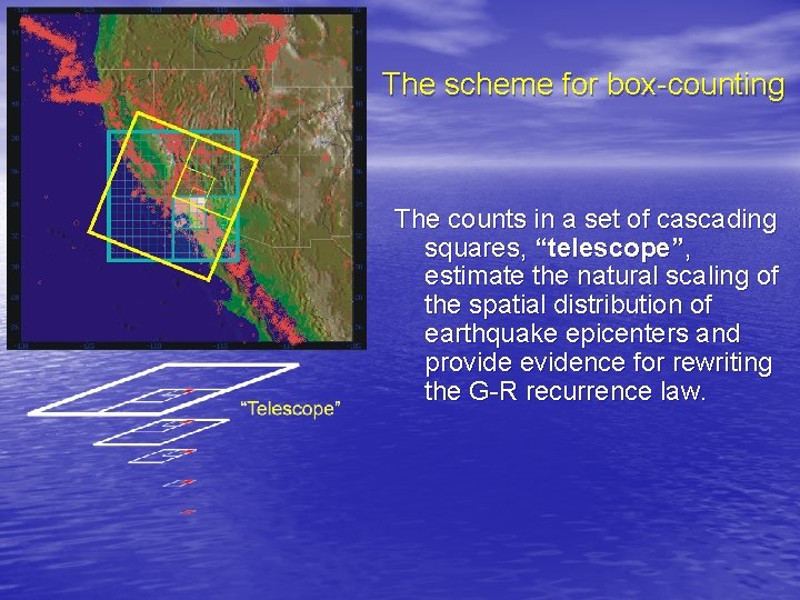
The scheme for box-counting The counts in a set of cascading squares, “telescope”, estimate the natural scaling of the spatial distribution of earthquake epicenters and provide evidence for rewriting the G-R recurrence law.

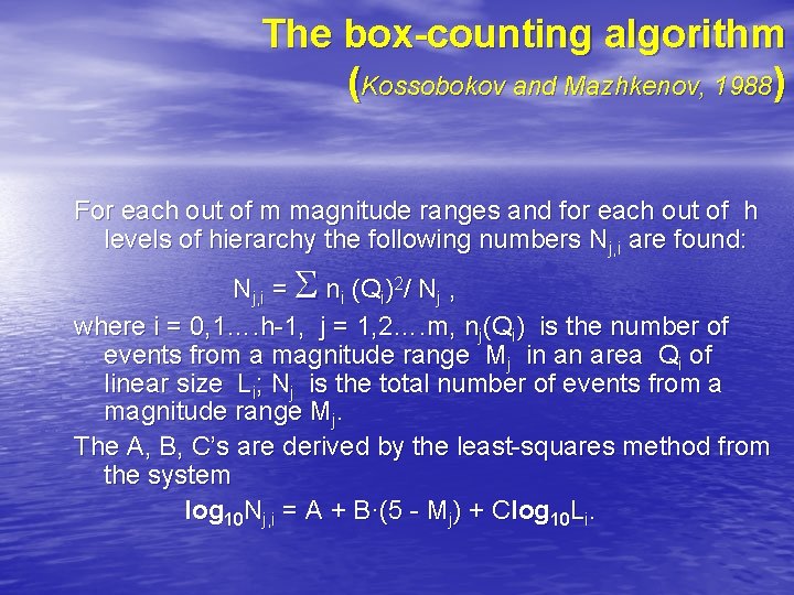
The box-counting algorithm (Kossobokov and Mazhkenov, 1988) For each out of m magnitude ranges and for each out of h levels of hierarchy the following numbers Nj, i are found: Nj, i = S ni (Qi)2/ Nj , where i = 0, 1…. h-1, j = 1, 2…. m, nj(Qi) is the number of events from a magnitude range Mj in an area Qi of linear size Li; Nj is the total number of events from a magnitude range Mj. The A, B, C’s are derived by the least-squares method from the system log 10 Nj, i = A + B·(5 - Mj) + Clog 10 Li.

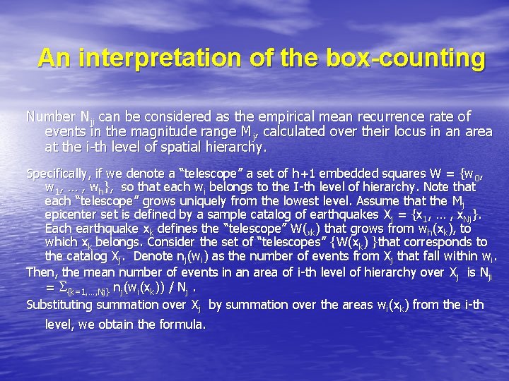
An interpretation of the box-counting Number Nji can be considered as the empirical mean recurrence rate of events in the magnitude range Mj, calculated over their locus in an area at the i-th level of spatial hierarchy. Specifically, if we denote a “telescope” a set of h+1 embedded squares W = {w 0, w 1, … , wh}, so that each wi belongs to the I-th level of hierarchy. Note that each “telescope” grows uniquely from the lowest level. Assume that the Mj epicenter set is defined by a sample catalog of earthquakes Xj = {x 1, … , x. Nj}. Each earthquake xk defines the “telescope” W(xk) that grows from wh(xk), to which xk belongs. Consider the set of “telescopes” {W(xk) }that corresponds to the catalog Xj. Denote nj(wi) as the number of events from Xj that fall within wi. Then, the mean number of events in an area of i-th level of hierarchy over Xj is Nji = S{k=1, …, Nj} nj(wi(xk)) / Nj. Substituting summation over Xj by summation over the areas wi(xk) from the i-th level, we obtain the formula.

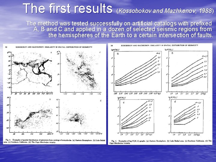
The first results (Kossobokov and Mazhkenov, 1988) The method was tested successfully on artificial catalogs with prefixed A, B and C and applied in a dozen of selected seismic regions from the hemispheres of the Earth to a certain intersection of faults.

The global map of the USLE coefficients: Recurrence ( A ) Logarithm of recurrence Year -1

The global map of the USLE coefficients: Balance of magnitudes ( B ) Balance between magnitude ranges Unit of magnitude-1

The global map of the USLE coefficients: Fractal dimension of seismic skeleton ( C ) Fractal dimension of epicenters

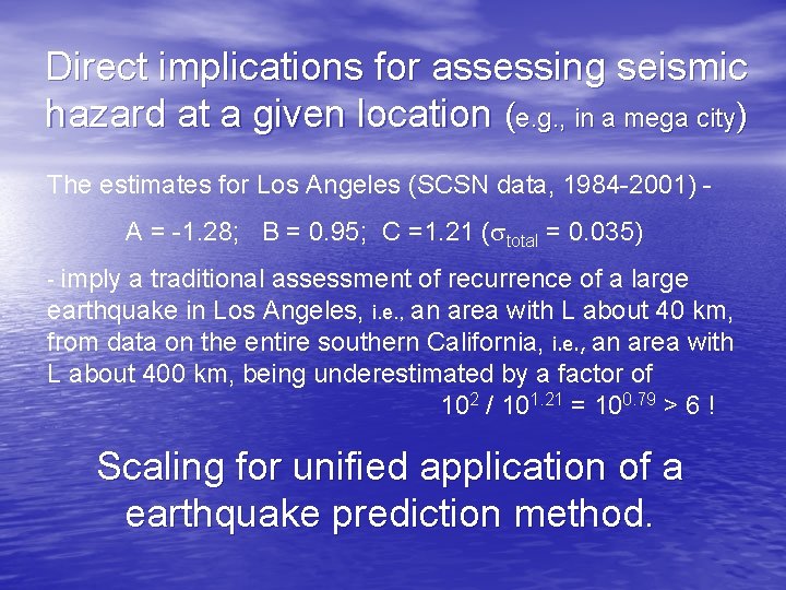
Direct implications for assessing seismic hazard at a given location (e. g. , in a mega city) The estimates for Los Angeles (SCSN data, 1984 -2001) A = -1. 28; B = 0. 95; C =1. 21 (stotal = 0. 035) imply a traditional assessment of recurrence of a large earthquake in Los Angeles, i. e. , an area with L about 40 km, from data on the entire southern California, i. e. , an area with L about 400 km, being underestimated by a factor of 102 / 101. 21 = 100. 79 > 6 ! - Scaling for unified application of a earthquake prediction method.

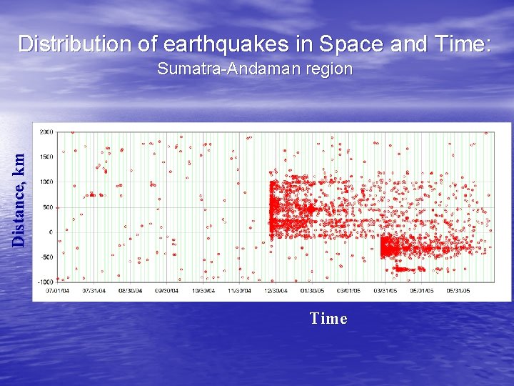
Distribution of earthquakes in Space and Time: Distance, km Sumatra-Andaman region Time

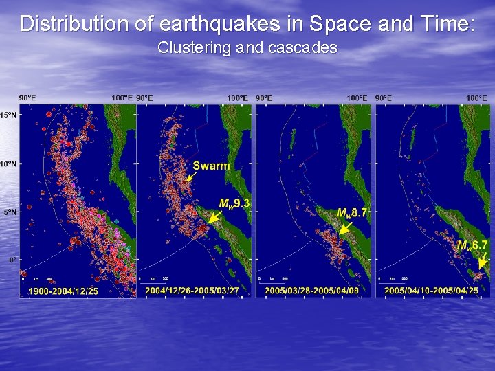
Distribution of earthquakes in Space and Time: Clustering and cascades

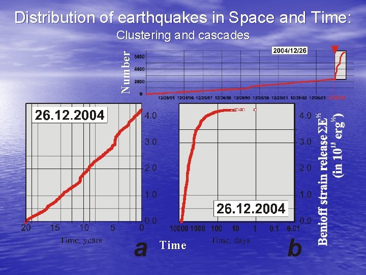
Distribution of earthquakes in Space and Time: Number Clustering and cascades Time

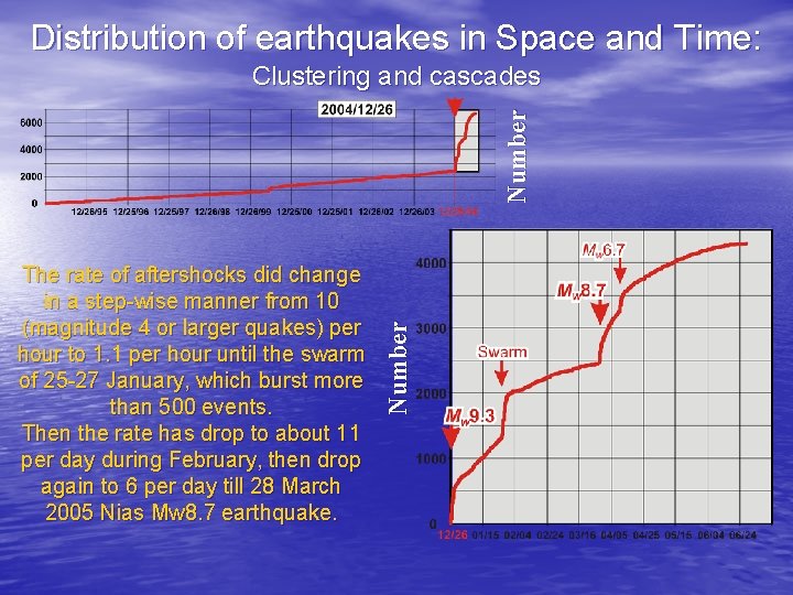
Distribution of earthquakes in Space and Time: The rate of aftershocks did change in a step-wise manner from 10 (magnitude 4 or larger quakes) per hour to 1. 1 per hour until the swarm of 25 -27 January, which burst more than 500 events. Then the rate has drop to about 11 per day during February, then drop again to 6 per day till 28 March 2005 Nias Mw 8. 7 earthquake. Number Clustering and cascades

Distribution of earthquakes in Space and Time: Inter-event time, days Clustering and cascades Lines are 20 per moving average of the inter-event time in an aftershock zone: 26 Dec 04 (red) 28 Mar 05 (blue) 10 Apr 05 (yellow) Time

Epoch analysis of aftershocks (evidence from southern CA) Aftershock sequences of southern California are extremely different – e. g. the total number of M 2. 0+ aftershocks in 100 days can be 0 for some main shocks up to magnitude 5. 0 (about 10 -25% of the total for different magnitudes) and can differ by a factor 10 or more for magnitude 6. 0 main shocks (for Whittier Narrows, 1987, M 6. 2, the number of M 2. 0+ aftershocks is about one hundred, while for Joshua thatit itis is widely used in conceptual models Tree, despite 1992, M 6. 1, above 19 hundred). For M 7. 0+, the recent Landers, 1992, M 7. 3, has about 8. 5 thousand, while Hector Mine, 1999, M 7. 1, has only 4. 6 thousand of M 2. 0+ aftershocks. Therefore, epoch analysis of the aftershock series is analogous to measuring of the average patients’ temperature in a clinic, while “an average behavior of the seismicity” in the region is analogous to crossing the pond through the middle of its waters, which is the average of walking around it, either by turning to the left or to the right. Thus, the “old good” Omori’s law for aftershocks is hardly a solidly documented fact ( ).

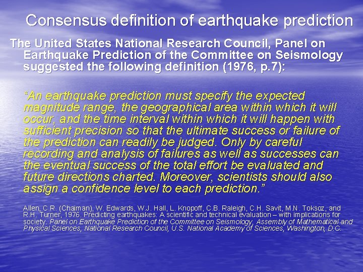
Consensus definition of earthquake prediction The United States National Research Council, Panel on Earthquake Prediction of the Committee on Seismology suggested the following definition (1976, p. 7): “An earthquake prediction must specify the expected magnitude range, the geographical area within which it will occur, and the time interval within which it will happen with sufficient precision so that the ultimate success or failure of the prediction can readily be judged. Only by careful recording and analysis of failures as well as successes can the eventual success of the total effort be evaluated and future directions charted. Moreover, scientists should also assign a confidence level to each prediction. ” Allen, C. R. (Chaiman), W. Edwards, W. J. Hall, L. Knopoff, C. B. Raleigh, C. H. Savit, M. N. Toksoz, and R. H. Turner, 1976. Predicting earthquakes: A scientific and technical evaluation – with implications for society. Panel on Earthquake Prediction of the Committee on Seismology, Assembly of Mathematical and Physical Sciences, National Research Council, U. S. National Academy of Sciences, Washington, D. C.

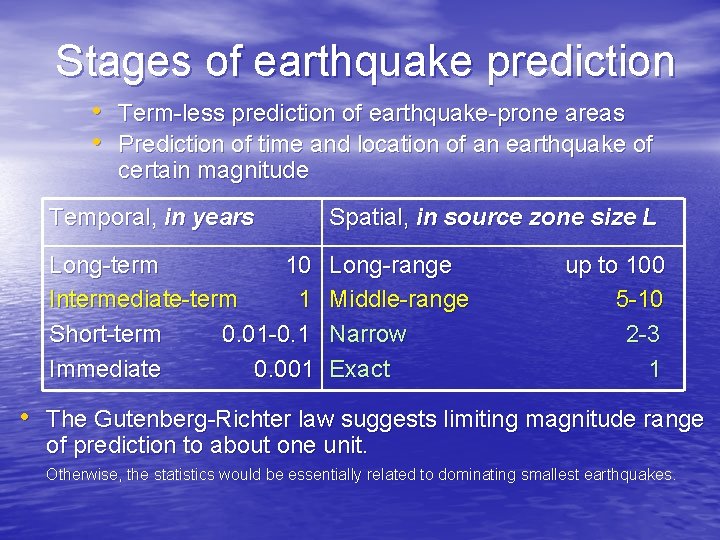
Stages of earthquake prediction • Term-less prediction of earthquake-prone areas • Prediction of time and location of an earthquake of certain magnitude Temporal, in years Spatial, in source zone size L Long-term 10 Intermediate-term 1 Short-term 0. 01 -0. 1 Immediate 0. 001 Long-range up to 100 Middle-range 5 -10 Narrow 2 -3 Exact 1 • The Gutenberg-Richter law suggests limiting magnitude range of prediction to about one unit. Otherwise, the statistics would be essentially related to dominating smallest earthquakes.

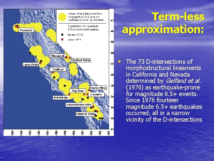
Term-less approximation: • The 73 D-intersections of morphostructural lineaments in California and Nevada determined by Gelfand et al. (1976) as earthquake-prone for magnitude 6. 5+ events. Since 1976 fourteen magnitude 6. 5+ earthquakes occurred, all in a narrow vicinity of the D-intersections

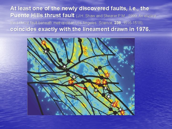
At least one of the newly discovered faults, i. e. , the Puente Hills thrust fault (J. H. Shaw and Shearer P. M. , 1999. An elusive blind-thrust fault beneath metropolitan Los Angeles. Science, 238, 1516 -1518), coincides exactly with the lineament drawn in 1976.

PLANETS ALIGN: On Wednesday morning, September 24 th, 2003 a lovely trio appeared in the eastern sky: Jupiter, the crescent moon and Mercury… Is it a coincidence or a law? Two days later … 防災科研Hi-net暫定処理による震源位置 本震 2003年 9月26日 04時50 分11秒 北緯 42. 0度 東経143. 9度 深さ 25 km M 7. 7 最大余震 2003年 9月26日 06時08 分03秒 北緯 41. 8度 東経143. 9度 深さ 35 km M 7. 4

• One or even a few observations is not • enough to claim causality and reject the alternative of coincidence by chance. Probability theory helps when a long series of observations permits to suggest a suitable probability model.

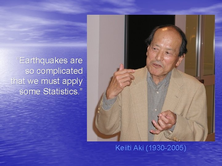
“Earthquakes are so complicated that we must apply some Statistics. ” Keiiti Aki (1930 -2005)

“Data consist of numbers, of course. But these numbers are fed into the computer, not produced by it. These numbers to be treated with considerable respect, neither to be tampered with, nor subjected to a numerical process whose character you do not completely understand. You are well advised to acquire a reverence for data that is rather different from the "sporty" attitude that is sometimes allowable, or even commendable, in other numerical tasks. … (William H. Press et al. , Numerical Recipes, p. 603)

… The analysis of data inevitably involves some trafficking with the field of statistics, that gray area which is not quite a branch of mathematics - and just as surely not quite a branch of science. In the following sections, you will repeatedly encounter the following paradigm: • apply some formula to the data to compute "a statistic" • compute where the value of that statistic falls in a probability distribution that is computed on the basis of some "null hypothesis" • if it falls in a very unlikely spot, way out on a tail of the distribution, conclude that the null hypothesis is false for your data set. … (William H. Press et al. , Numerical Recipes, p. 603)

… If a statistic falls in a reasonable part of the distribution, you must not make the mistake of concluding that the null hypothesis is "verified" or "proved". That is the curse of statistics, that it can never prove things, only disprove them! At best, you can substantiate a hypothesis by ruling out, statistically, a whole long list of competing hypotheses, every one that has ever been proposed. After a while your adversaries and competitors will give up trying to think of alternative hypotheses, or else they will grow old and die, and then your hypothesis will become accepted. Sounds crazy, we know, but that's how science works!” (William H. Press et al. , Numerical Recipes, p. 603)

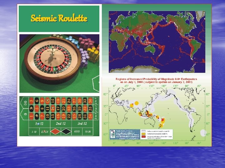
Seismic Roulette

Seismic Roulette • • • Consider a roulette wheel with as many sectors as the number of events in a sample catalog, a sector per each event. Make your bet according to prediction: determine, which events are inside area of alarm, and put one chip in each of the corresponding sectors. Nature turns the wheel. If seismic roulette is not perfect… then systematically you can win! and lose … If you are smart enough and your predictions are effective -----the first will outscore the second!

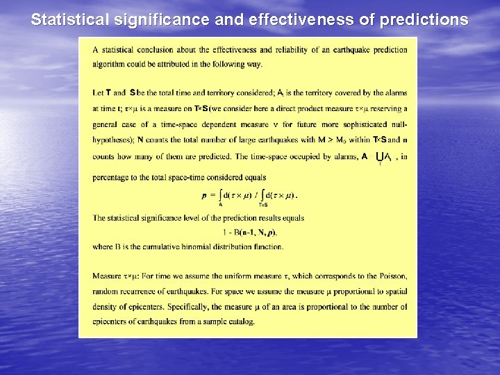
Statistical significance and effectiveness of predictions

This simple comparison with random guessing apply to any prediction method • GAP theory • Quiescence hypothesis • the VAN method • the Jackson-Kagan forecast probability maps • the Kushida method • etc Surprisingly, most of the authors seem avoiding real-time testing, evaluation and verification…

How earthquake prediction methods work? “Predicting earthquakes is as easy as one-twothree. • Step 1: Deploy your precursor detection instruments at the site of the coming earthquake. Routine seismological data bases, e. g. US GS/NEIC • Step 2: Detect and recognize the precursors. Reproducible intermediate-term algorithms, e. g. M 8 • Step 3: Get all your colleagues to agree and then publicly predict the earthquake through approved Number of earthquakes have been predicted channels. ” Scholz, C. H. , 1997. Whatever happened to earthquake prediction. Geotimes, 42(3), 16 -19

(available from IASPEI Software Library, Vol. 6. Seismol. Soc. Am. , El Cerrito, CA, 1997) M 8 algorithm This intermediate-term earthquake prediction method was designed by retroactive analysis of dynamics of seismic activity preceding the greatest, magnitude 8. 0 or more, earthquakes worldwide, hence its name. Its prototype (Keilis-Borok and Kossobokov, 1984) and the original version (Keilis-Borok and Kossobokov, 1987) were tested retroactively. The original version of M 8 is subject to the on-going real-time experimental testing. After a decade the results confirm predictability of the great earthquakes beyond any reasonable doubt. The algorithm is based on a simple physical scheme…

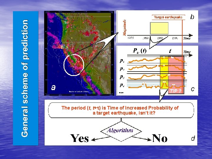
The period (t, t+t) is Time of Increased Probability of a target earthquake, isn’t it?

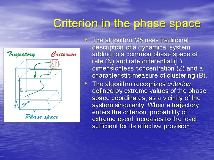
Criterion in the phase space • The algorithm M 8 uses traditional • description of a dynamical system adding to a common phase space of rate (N) and rate differential (L) dimensionless concentration (Z) and a characteristic measure of clustering (B). The algorithm recognizes criterion, defined by extreme values of the phase space coordinates, as a vicinity of the system singularity. When a trajectory enters the criterion, probability of extreme event increases to the level sufficient for its effective provision.

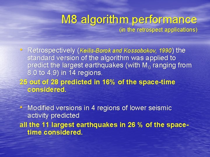
M 8 algorithm performance (in the retrospect applications) • Retrospectively (Keilis-Borok and Kossobokov, 1990) the standard version of the algorithm was applied to predict the largest earthquakes (with M 0 ranging from 8. 0 to 4. 9) in 14 regions. 25 out of 28 predicted in 16% of the space-time considered. • Modified versions in 4 regions of lower seismic activity predicted all the 11 largest earthquakes in 26 % of the spacetime considered.

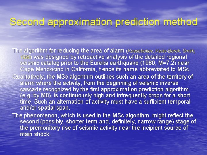
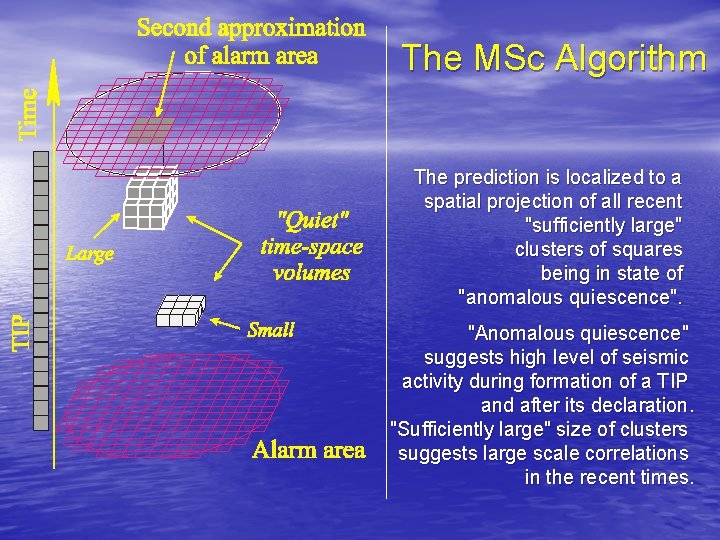
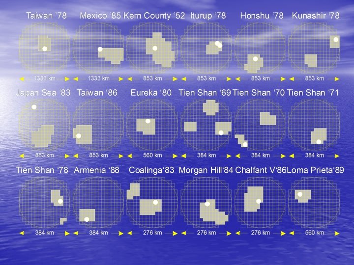
Second approximation prediction method The algorithm for reducing the area of alarm (Kossobokov, Keilis-Borok, Smith, 1990) was designed by retroactive analysis of the detailed regional seismic catalog prior to the Eureka earthquake (1980, M=7. 2) near Cape Mendocino in California, hence its name abbreviated to MSc. Qualitatively, the MSc algorithm outlines such an area of the territory of alarm where the activity, from the beginning of seismic inverse cascade recognized by the first approximation prediction algorithm (e. g. by M 8), is continuously high and infrequently drops for a short time. Such an alternation of activity must have a sufficient temporal and/or spatial span. The phenomenon, which is used in the MSc algorithm, might reflect the second (possibly, shorter-term and, definitely, narrow-range) stage of the premonitory rise of seismic activity near the incipient source of main shock.

The MSc Algorithm The prediction is localized to a spatial projection of all recent "sufficiently large" clusters of squares being in state of "anomalous quiescence". "Anomalous quiescence" suggests high level of seismic activity during formation of a TIP and after its declaration. "Sufficiently large" size of clusters suggests large scale correlations in the recent times.

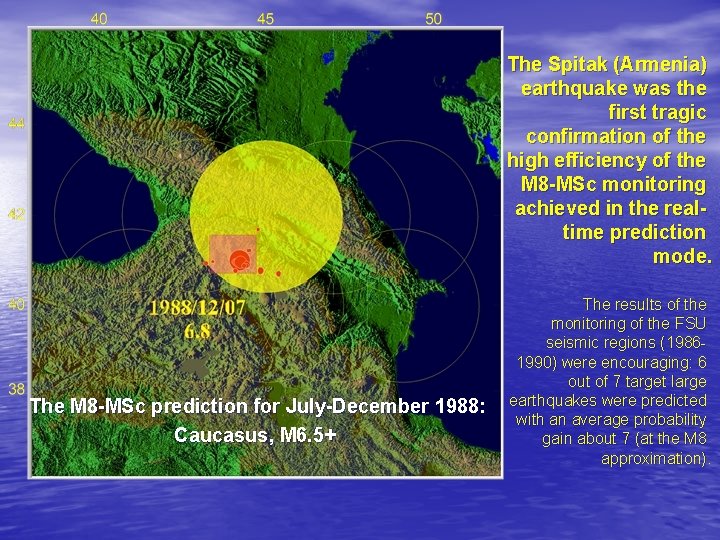
The Spitak (Armenia) earthquake was the first tragic confirmation of the high efficiency of the M 8 -MSc monitoring achieved in the realtime prediction mode. The M 8 -MSc prediction for July-December 1988: Caucasus, M 6. 5+ The results of the monitoring of the FSU seismic regions (19861990) were encouraging: 6 out of 7 target large earthquakes were predicted with an average probability gain about 7 (at the M 8 approximation).

By 1992 all the components necessary for reproducible real-time prediction, i. e. , an unambiguous definition of the algorithms and the data base, were specified in publications • Algorithm M 8 (Keilis-Borok and Kossobokov, 1984, 1987, 1990) • • was designed by retroactive analysis of seismic dynamics preceding the greatest (M 8) earthquakes worldwide, as well as the MSc algorithm for reducing the area of alarm (Kossobokov, Keilis-Borok, Smith, 1990) The National Earthquake Information Center Global Hypocenters Data Base (US GS/NEIC GHDB, 1989) is sufficiently complete since 1963. This allowed a systematic application of M 8 and MSc algorithm since 1985.

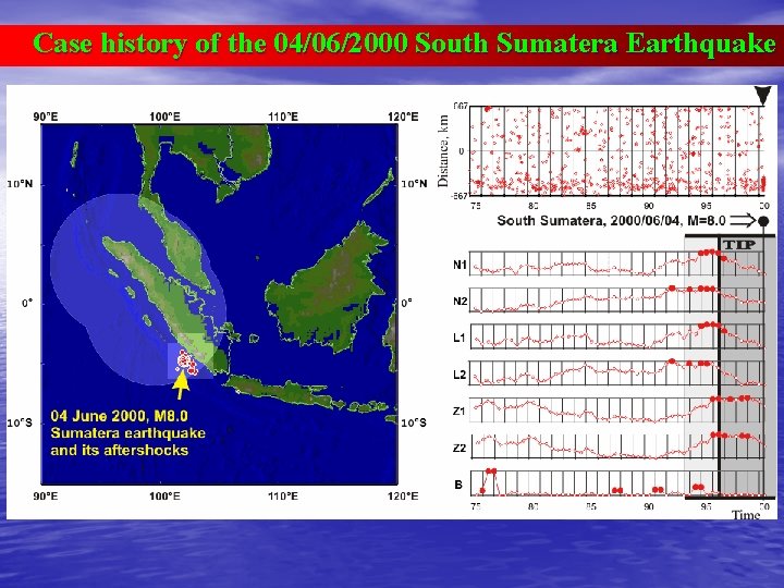
Case history of the 04/06/2000 South Sumatera Earthquake

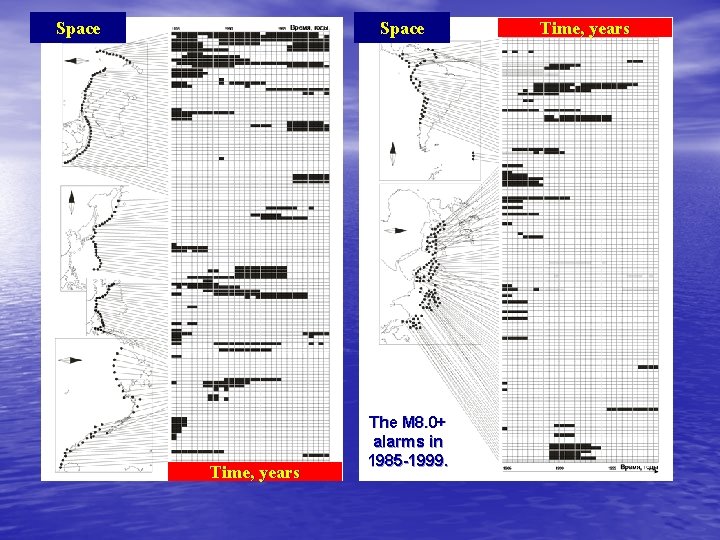
Space Time, years The M 8. 0+ alarms in 1985 -1999. Time, years

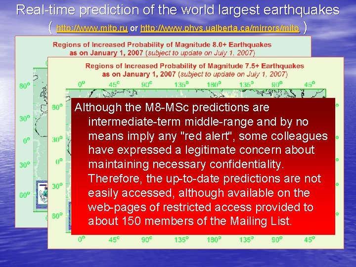
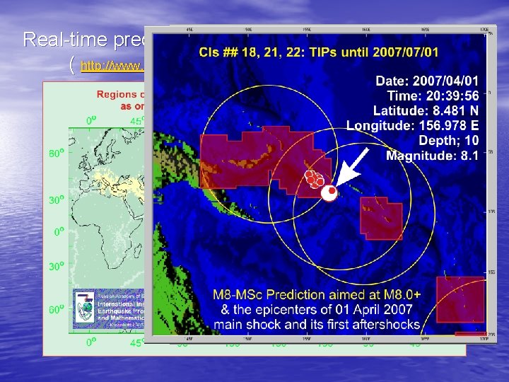
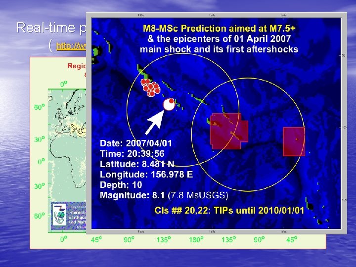
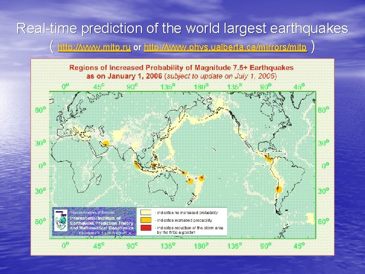
Real-time prediction of the world largest earthquakes ( http: //www. mitp. ru or http: //www. phys. ualberta. ca/mirrors/mitp ) Although the M 8 -MSc predictions are intermediate-term middle-range and by no means imply any "red alert", some colleagues have expressed a legitimate concern about maintaining necessary confidentiality. Therefore, the up-to-date predictions are not easily accessed, although available on the web-pages of restricted access provided to about 150 members of the Mailing List.

Real-time prediction of the world largest earthquakes ( http: //www. mitp. ru or http: //www. phys. ualberta. ca/mirrors/mitp )

Real-time prediction of the world largest earthquakes ( http: //www. mitp. ru or http: //www. phys. ualberta. ca/mirrors/mitp )

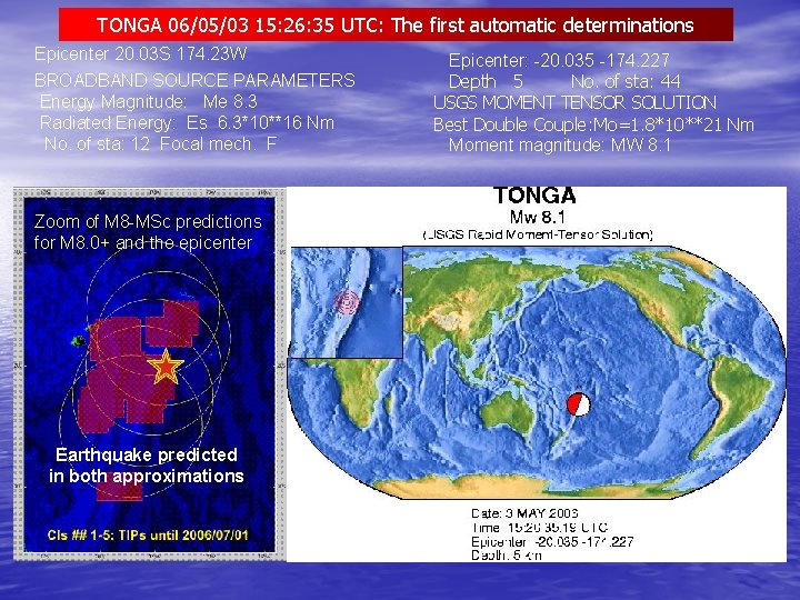
TONGA 06/05/03 15: 26: 35 UTC: The first automatic determinations Epicenter 20. 03 S 174. 23 W BROADBAND SOURCE PARAMETERS Energy Magnitude: Me 8. 3 Radiated Energy: Es 6. 3*10**16 Nm No. of sta: 12 Focal mech. F Zoom of M 8 -MSc predictions for M 8. 0+ and the epicenter Earthquake predicted in both approximations Epicenter: -20. 035 -174. 227 Depth 5 No. of sta: 44 USGS MOMENT TENSOR SOLUTION Best Double Couple: Mo=1. 8*10**21 Nm Moment magnitude: MW 8. 1

Real-time prediction of the world largest earthquakes ( http: //www. mitp. ru or http: //www. phys. ualberta. ca/mirrors/mitp )

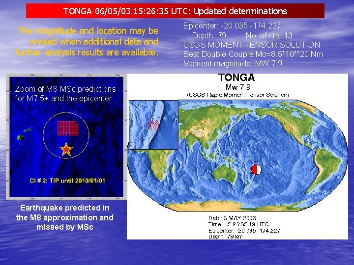
TONGA 06/05/03 15: 26: 35 UTC: Updated determinations The magnitude and location may be revised when additional data and further analysis results are available. Zoom of M 8 -MSc predictions for M 7. 5+ and the epicenter Earthquake predicted in the M 8 approximation and missed by MSc Epicenter: -20. 035 -174. 227 Depth 79 No. of sta: 13 USGS MOMENT TENSOR SOLUTION Best Double Couple: Mo=8. 5*10**20 Nm Moment magnitude: MW 7. 9

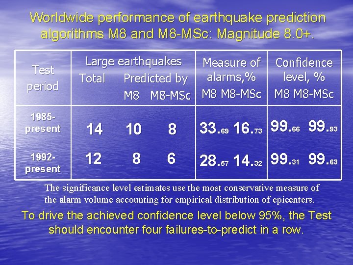
Worldwide performance of earthquake prediction algorithms M 8 and M 8 -MSc: Magnitude 8. 0+. Test period 1985 present 1992 present Large earthquakes Measure of alarms, % Total Predicted by M 8 M 8 -MSc Confidence level, % M 8 -MSc 14 10 8 33. 69 16. 73 99. 66 99. 93 12 8 6 28. 57 14. 32 99. 31 99. 63 The significance level estimates use the most conservative measure of the alarm volume accounting for empirical distribution of epicenters. To drive the achieved confidence level below 95%, the Test should encounter four failures-to-predict in a row.

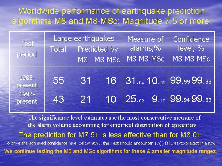
Worldwide performance of earthquake prediction algorithms M 8 and M 8 -MSc: Magnitude 7. 5 or more. Test period 1985 present 1992 present Large earthquakes Measure of alarms, % Total Predicted by M 8 M 8 -MSc Confidence level, % M 8 -MSc 55 31 16 31. 10. 99 99. 99 04 05 43 21 10 25. 9. 94 99. 55 02 10 The significance level estimates use the most conservative measure of the alarm volume accounting for empirical distribution of epicenters. The prediction for M 7. 5+ is less effective than for M 8. 0+. To drive the achieved confidence level below 95%, the Test should encounter 17(!) failures-to-predict in a row. We continue testing the M 8 and MSc algorithms for these & smaller magnitude ranges.

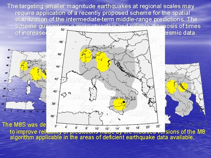
The targeting smaller magnitude earthquakes at regional scales may require application of a recently proposed scheme for the spatial stabilization of the intermediate-term middle-range predictions. The scheme guarantees a more objective and reliable diagnosis of times of increased probability and is less restrictive to input seismic data. The M 8 S was designed originally to improve reliability of predictions made by the modified versions of the M 8 algorithm applicable in the areas of deficient earthquake data available.

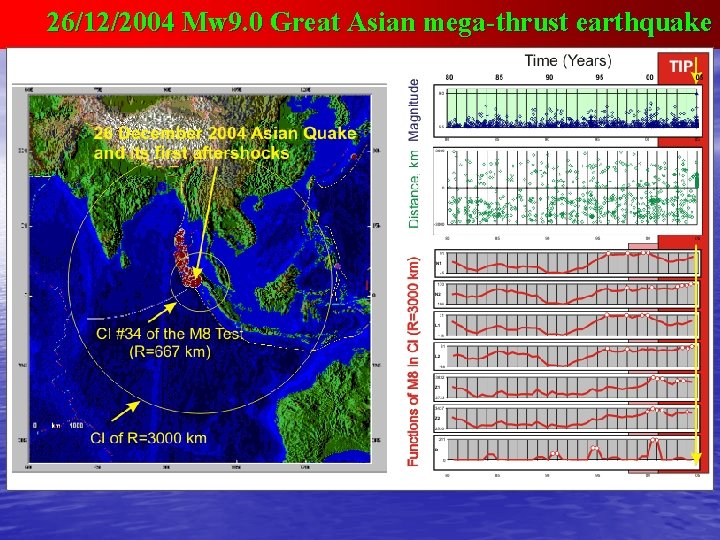
The recent disaster in Indian Ocean If on July 1, 2004 someone had been sufficiently ambitious to extend application of the M 8 algorithm into the uncalibrated magnitude range targeting M 9. 0+ earthquakes, he or she would have diagnosed Time of Increased Probability in advance of the 2004 Great Asian Quake. Unfortunately, in the on-going Global Testing of M 8 -MSc predictions aimed at M 8. 0+ events, it was a case of one not being able to see the forest for the trees. The December 26 event seems to be the first indication that the algorithm, designed for prediction of M 8. 0+ earthquakes can be rescaled for prediction of both smaller magnitude earthquakes (e. g. , down to M 5. 5+ in Italy http: //www. mitp. ru/m 8 s/M 8 s_italy. html) and for mega-earthquakes of M 9. 0+. The event is not full verification, but very important for general understanding of our methodology (Nonlinear Dynamics of the Lithosphere and Earthquake Prediction. Keilis-Borok, V. I. , & A. A. Soloviev (Eds). Springer, Heidelberg, 2003) and the Problem of Earthquake Prediction.

26/12/2004 Mw 9. 0 Great Asian mega-thrust earthquake

The relevant observation: All the largest four mega-earthquakes of the 20 th century (Kamchatka, 1952/11/04, Mw 9. 0; Andreanoff Islands, 1957/03/09, Mw 9. 1; Chile, 1960/05/22, Mw 9. 5; Alaska, 1964/03/28, Mw 9. 2) happened within a narrow interval of time. Such a cluster is unlikely with a 99% confidence for uniformly distributed independent events. Since good evidence suggests that seismic events including mega-earthquakes cluster, it is possible that we will have further confirmation of the prediction within 5 -10 years in other regions. The 28 March 2005 Nias Mw 8. 7 mega-earthquake seems to be the first confirmation.

Conclusions – The Four Paradigms Statistical validity of predictions confirms the underlying paradigms: • Seismic premonitory patterns exist; • Formation of earthquake precursors at scale of years involves large size fault system; • The phenomena are similar in a wide range of tectonic environment… • … and in other complex non-linear systems.

Conclusions – Seismic Roulette is not perfect Are these predictions useful? • Yes, if used in a knowledgeable way. • Their accuracy is already enough for undertaking earthquake preparedness measures, which would prevent a considerable part of damage and human loss, although far from the total. • The methodology linking prediction with disaster management strategies does exist (Molchan, 1997).

Conclusions – Implications for Physics • The predictions provide reliable empirical • • constrains for modeling earthquakes and earthquake sequences. Evidence that distributed seismic activity is a problem in statistical physics. Favor the hypothesis that earthquakes follow a general hierarchical process that proceeds via a sequence of inverse cascades to produce selfsimilar scaling (intermediate asymptotic), which then truncates at the largest scales bursting into direct cascades (Gabrielov, Newman, Turcotte, 1999).

What are the Next Steps? • The algorithms are neither optimal nor unique (CN, SSE, Vere-Jones “probabilistic” version of M 8, RTP, R. E. L. M. , E. T. A. S. , “hot spots”, etc. ). Their non-randomness could be checked and their accuracy could be improved by a systematic monitoring of the alarm areas and by designing a new generation of earthquake prediction technique. … and an obvious general one • More data should be analyzed systematically to establish reliable correlations between the occurrence of extreme events and observable phenomena.

Thank you