Utility Maximization and Choice Power Point Slides prepared

Utility Maximization and Choice Power. Point Slides prepared by: Andreea CHIRITESCU, Eastern Illinois University; Modified by: Ronald WENDNER, University of Graz, Austria © 2012 Cengage Learning. All Rights Reserved. May not be copied, scanned, or duplicated, in whole or in part, except for use as permitted in a license distributed with a certain product or service or otherwise on a password-protected website for classroom use. 1

The Plan • Utility maximization (☞ Marshallian demand) • Two-good case • N-good case • Indirect utility function • Expenditure minimization (☞ Hicksian demand) • Expenditure function © 2012 Cengage Learning. All Rights Reserved. May not be copied, scanned, or duplicated, in whole or in part, except for use as permitted in a license distributed with a certain product or service or otherwise on a password-protected website for classroom use. 2

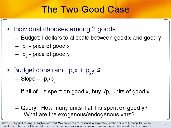
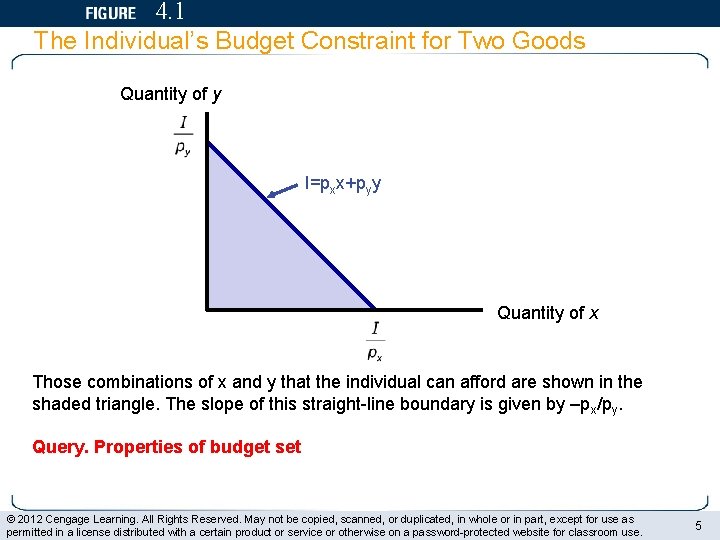
The Two-Good Case • Individual chooses among 2 goods – Budget: I dollars to allocate between good x and good y – px - price of good x – py - price of good y • Budget constraint: pxx + pyy ≤ I – Slope = -px/py – If all of I is spent on good x, buy I/px units of good x – Query: How many units if all I is spent on good y? What are the exogenous/endogenous vars? © 2012 Cengage Learning. All Rights Reserved. May not be copied, scanned, or duplicated, in whole or in part, except for use as permitted in a license distributed with a certain product or service or otherwise on a password-protected website for classroom use. 4

4. 1 The Individual’s Budget Constraint for Two Goods Quantity of y I=pxx+pyy Quantity of x Those combinations of x and y that the individual can afford are shown in the shaded triangle. The slope of this straight-line boundary is given by –px/py. Query. Properties of budget set © 2012 Cengage Learning. All Rights Reserved. May not be copied, scanned, or duplicated, in whole or in part, except for use as permitted in a license distributed with a certain product or service or otherwise on a password-protected website for classroom use. 5

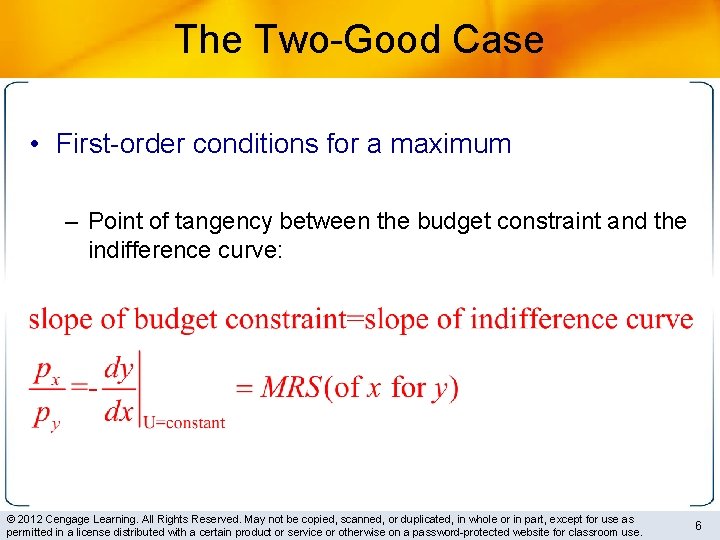
The Two-Good Case • First-order conditions for a maximum – Point of tangency between the budget constraint and the indifference curve: © 2012 Cengage Learning. All Rights Reserved. May not be copied, scanned, or duplicated, in whole or in part, except for use as permitted in a license distributed with a certain product or service or otherwise on a password-protected website for classroom use. 6

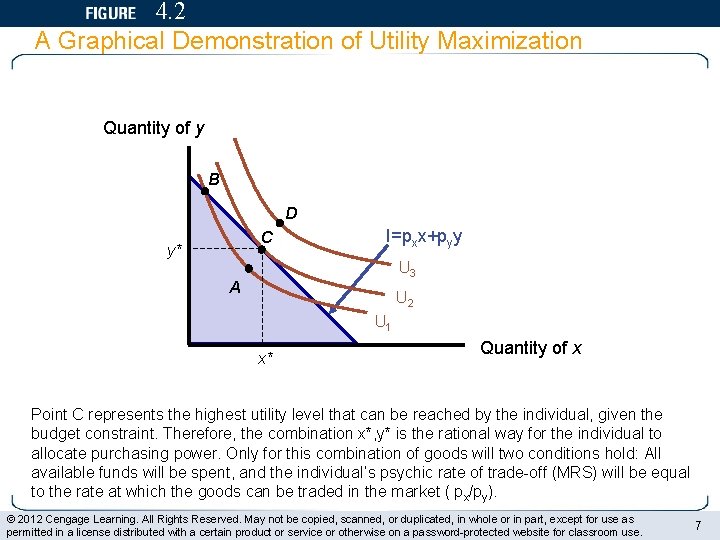
4. 2 A Graphical Demonstration of Utility Maximization Quantity of y B D C y* I=pxx+pyy U 3 A U 2 U 1 x* Quantity of x Point C represents the highest utility level that can be reached by the individual, given the budget constraint. Therefore, the combination x*, y* is the rational way for the individual to allocate purchasing power. Only for this combination of goods will two conditions hold: All available funds will be spent, and the individual’s psychic rate of trade-off (MRS) will be equal to the rate at which the goods can be traded in the market ( px/py). © 2012 Cengage Learning. All Rights Reserved. May not be copied, scanned, or duplicated, in whole or in part, except for use as permitted in a license distributed with a certain product or service or otherwise on a password-protected website for classroom use. 7

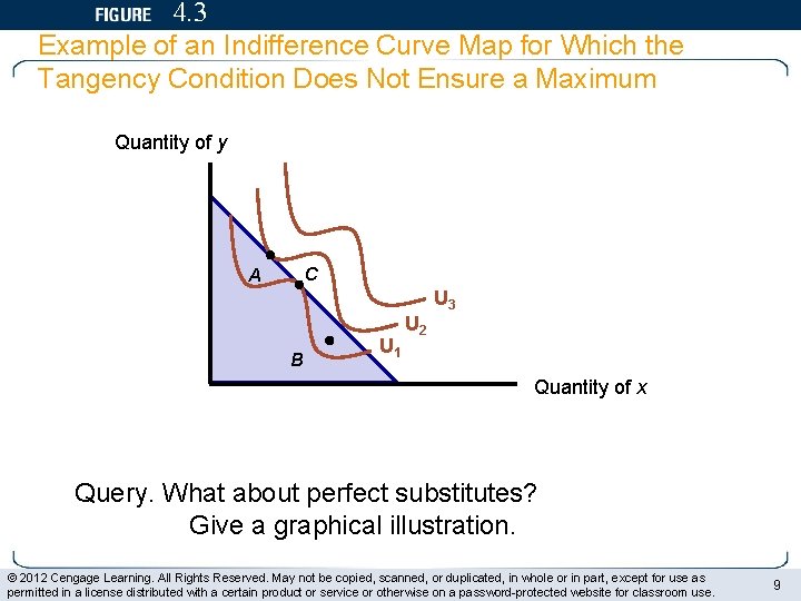
The Two-Good Case • The tangency rule – Is not sufficient • If MRS is not diminishing, we must check second-order conditions to ensure that we are at a maximum • What about points A and D in the previous figure? – Query. Is tangency rule necessary? © 2012 Cengage Learning. All Rights Reserved. May not be copied, scanned, or duplicated, in whole or in part, except for use as permitted in a license distributed with a certain product or service or otherwise on a password-protected website for classroom use. 8

4. 3 Example of an Indifference Curve Map for Which the Tangency Condition Does Not Ensure a Maximum Quantity of y C A B U 1 U 2 U 3 Quantity of x Query. What about perfect substitutes? Give a graphical illustration. © 2012 Cengage Learning. All Rights Reserved. May not be copied, scanned, or duplicated, in whole or in part, except for use as permitted in a license distributed with a certain product or service or otherwise on a password-protected website for classroom use. 9

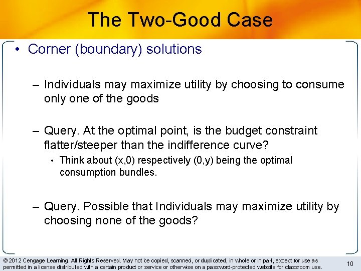
The Two-Good Case • Corner (boundary) solutions – Individuals may maximize utility by choosing to consume only one of the goods – Query. At the optimal point, is the budget constraint flatter/steeper than the indifference curve? • Think about (x, 0) respectively (0, y) being the optimal consumption bundles. – Query. Possible that Individuals may maximize utility by choosing none of the goods? © 2012 Cengage Learning. All Rights Reserved. May not be copied, scanned, or duplicated, in whole or in part, except for use as permitted in a license distributed with a certain product or service or otherwise on a password-protected website for classroom use. 10

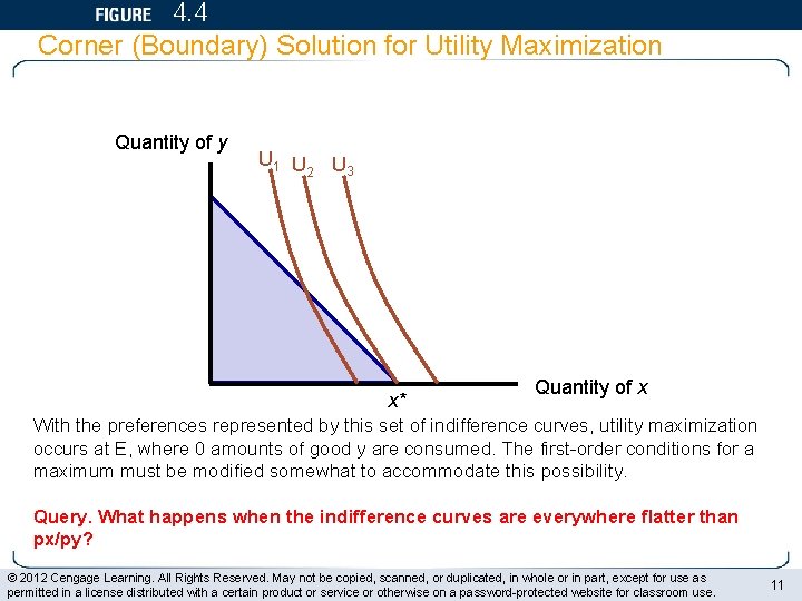
4. 4 Corner (Boundary) Solution for Utility Maximization Quantity of y U 1 U U 3 2 x* Quantity of x With the preferences represented by this set of indifference curves, utility maximization occurs at E, where 0 amounts of good y are consumed. The first-order conditions for a maximum must be modified somewhat to accommodate this possibility. Query. What happens when the indifference curves are everywhere flatter than px/py? © 2012 Cengage Learning. All Rights Reserved. May not be copied, scanned, or duplicated, in whole or in part, except for use as permitted in a license distributed with a certain product or service or otherwise on a password-protected website for classroom use. 11

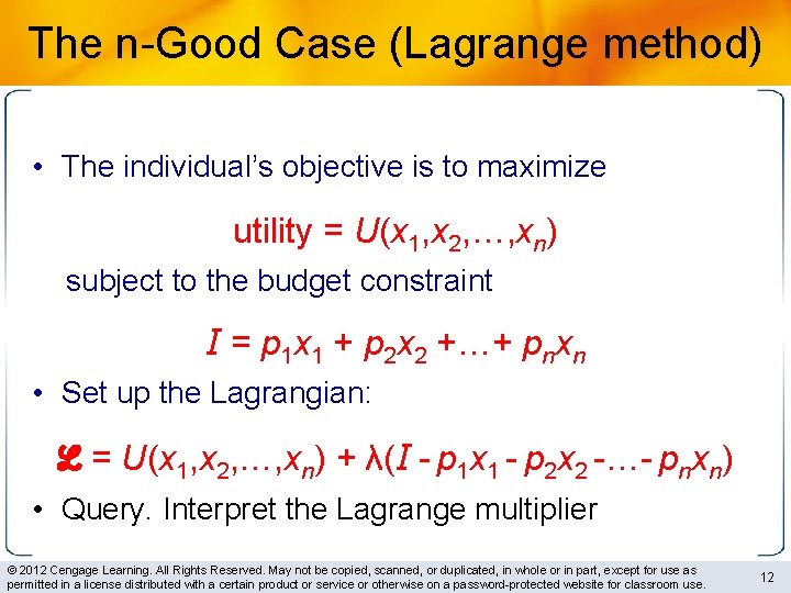
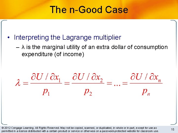
The n-Good Case (Lagrange method) • The individual’s objective is to maximize utility = U(x 1, x 2, …, xn) subject to the budget constraint I = p 1 x 1 + p 2 x 2 +…+ pnxn • Set up the Lagrangian: ℒ = U(x 1, x 2, …, xn) + λ(I - p 1 x 1 - p 2 x 2 -…- pnxn) • Query. Interpret the Lagrange multiplier © 2012 Cengage Learning. All Rights Reserved. May not be copied, scanned, or duplicated, in whole or in part, except for use as permitted in a license distributed with a certain product or service or otherwise on a password-protected website for classroom use. 12

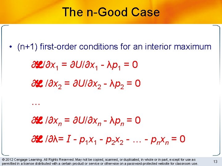
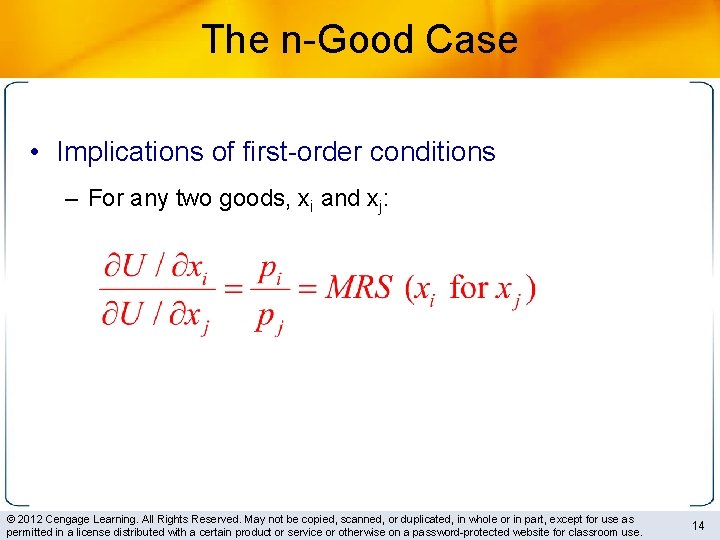
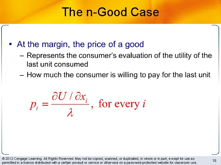
The n-Good Case • (n+1) first-order conditions for an interior maximum ∂ℒ/∂x 1 = ∂U/∂x 1 - λp 1 = 0 ∂ℒ /∂x 2 = ∂U/∂x 2 - λp 2 = 0 … ∂ℒ /∂xn = ∂U/∂xn - λpn = 0 ∂ℒ /∂λ= I - p 1 x 1 - p 2 x 2 - … - pnxn = 0 © 2012 Cengage Learning. All Rights Reserved. May not be copied, scanned, or duplicated, in whole or in part, except for use as permitted in a license distributed with a certain product or service or otherwise on a password-protected website for classroom use. 13

The n-Good Case • Implications of first-order conditions – For any two goods, xi and xj: © 2012 Cengage Learning. All Rights Reserved. May not be copied, scanned, or duplicated, in whole or in part, except for use as permitted in a license distributed with a certain product or service or otherwise on a password-protected website for classroom use. 14

The n-Good Case • Interpreting the Lagrange multiplier – λ is the marginal utility of an extra dollar of consumption expenditure (of income) © 2012 Cengage Learning. All Rights Reserved. May not be copied, scanned, or duplicated, in whole or in part, except for use as permitted in a license distributed with a certain product or service or otherwise on a password-protected website for classroom use. 15

The n-Good Case • © 2012 Cengage Learning. All Rights Reserved. May not be copied, scanned, or duplicated, in whole or in part, except for use as permitted in a license distributed with a certain product or service or otherwise on a password-protected website for classroom use. 16

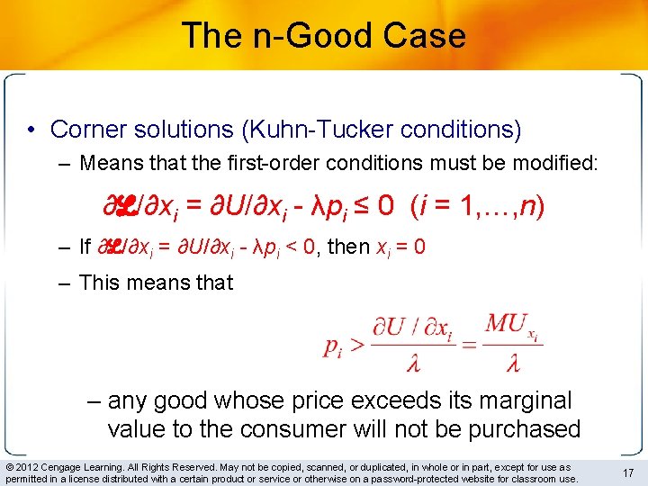
The n-Good Case • Corner solutions (Kuhn-Tucker conditions) – Means that the first-order conditions must be modified: ∂ℒ/∂xi = ∂U/∂xi - λpi ≤ 0 (i = 1, …, n) – If ∂ℒ/∂xi = ∂U/∂xi - λpi < 0, then xi = 0 – This means that – any good whose price exceeds its marginal value to the consumer will not be purchased © 2012 Cengage Learning. All Rights Reserved. May not be copied, scanned, or duplicated, in whole or in part, except for use as permitted in a license distributed with a certain product or service or otherwise on a password-protected website for classroom use. 17

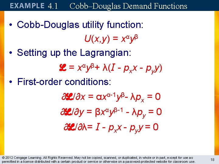
4. 1 Cobb–Douglas Demand Functions • Cobb-Douglas utility function: U(x, y) = xαyβ • Setting up the Lagrangian: ℒ = xαyβ+ λ(I - pxx - pyy) • First-order conditions: ∂ℒ/∂x = αxα-1 yβ- λpx = 0 ∂ℒ/∂y = βxαyβ-1 - λpy = 0 ∂ℒ/∂λ= I - pxx - pyy = 0 © 2012 Cengage Learning. All Rights Reserved. May not be copied, scanned, or duplicated, in whole or in part, except for use as permitted in a license distributed with a certain product or service or otherwise on a password-protected website for classroom use. 18

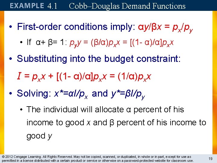
4. 1 Cobb–Douglas Demand Functions • First-order conditions imply: αy/βx = px/py • If α+ β= 1: pyy = (β/α)pxx = [(1 - α)/α]pxx • Substituting into the budget constraint: I = pxx + [(1 - α)/α]pxx = (1/α)pxx • Solving: x*=αI/px and y*=βI/py • The individual will allocate α percent of his income to good x and β percent of his income to good y © 2012 Cengage Learning. All Rights Reserved. May not be copied, scanned, or duplicated, in whole or in part, except for use as permitted in a license distributed with a certain product or service or otherwise on a password-protected website for classroom use. 19

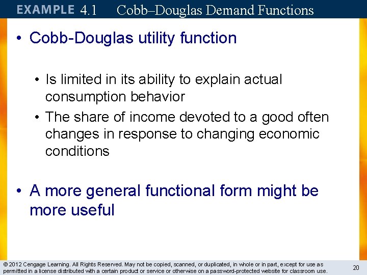
4. 1 Cobb–Douglas Demand Functions • Cobb-Douglas utility function • Is limited in its ability to explain actual consumption behavior • The share of income devoted to a good often changes in response to changing economic conditions • A more general functional form might be more useful © 2012 Cengage Learning. All Rights Reserved. May not be copied, scanned, or duplicated, in whole or in part, except for use as permitted in a license distributed with a certain product or service or otherwise on a password-protected website for classroom use. 20

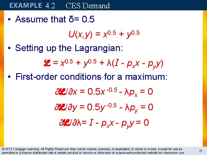
4. 2 CES Demand • Assume that δ= 0. 5 U(x, y) = x 0. 5 + y 0. 5 • Setting up the Lagrangian: ℒ = x 0. 5 + y 0. 5 + λ(I - pxx - pyy) • First-order conditions for a maximum: ∂ℒ/∂x = 0. 5 x -0. 5 - λpx = 0 ∂ℒ/∂y = 0. 5 y -0. 5 - λpy = 0 ∂ℒ/∂λ= I - pxx - pyy = 0 © 2012 Cengage Learning. All Rights Reserved. May not be copied, scanned, or duplicated, in whole or in part, except for use as permitted in a license distributed with a certain product or service or otherwise on a password-protected website for classroom use. 21

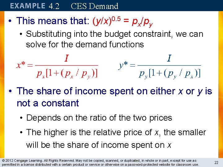
4. 2 CES Demand • This means that: (y/x)0. 5 = px/py • Substituting into the budget constraint, we can solve for the demand functions • The share of income spent on either x or y is not a constant • Depends on the ratio of the two prices • The higher is the relative price of x, the smaller will be the share of income spent on x © 2012 Cengage Learning. All Rights Reserved. May not be copied, scanned, or duplicated, in whole or in part, except for use as permitted in a license distributed with a certain product or service or otherwise on a password-protected website for classroom use. 22

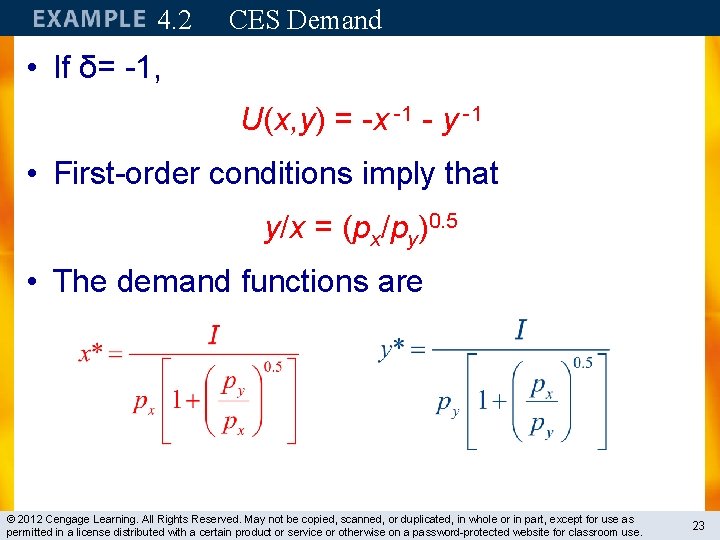
4. 2 CES Demand • If δ= -1, U(x, y) = -x -1 - y -1 • First-order conditions imply that y/x = (px/py)0. 5 • The demand functions are © 2012 Cengage Learning. All Rights Reserved. May not be copied, scanned, or duplicated, in whole or in part, except for use as permitted in a license distributed with a certain product or service or otherwise on a password-protected website for classroom use. 23

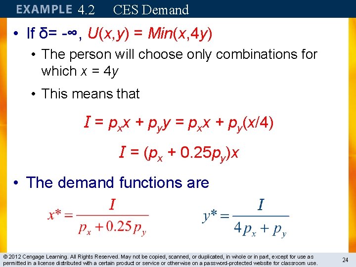
4. 2 CES Demand • If δ= -∞, U(x, y) = Min(x, 4 y) • The person will choose only combinations for which x = 4 y • This means that I = pxx + pyy = pxx + py(x/4) I = (px + 0. 25 py)x • The demand functions are © 2012 Cengage Learning. All Rights Reserved. May not be copied, scanned, or duplicated, in whole or in part, except for use as permitted in a license distributed with a certain product or service or otherwise on a password-protected website for classroom use. 24

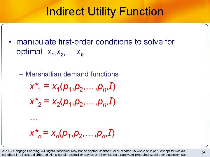
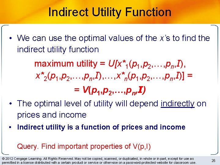
Indirect Utility Function • manipulate first-order conditions to solve for optimal x 1, x 2, …, xn – Marshallian demand functions x*1 = x 1(p 1, p 2, …, pn, I) x*2 = x 2(p 1, p 2, …, pn, I) … x*n = xn(p 1, p 2, …, pn, I) © 2012 Cengage Learning. All Rights Reserved. May not be copied, scanned, or duplicated, in whole or in part, except for use as permitted in a license distributed with a certain product or service or otherwise on a password-protected website for classroom use. 25

Indirect Utility Function • We can use the optimal values of the x’s to find the indirect utility function maximum utility = U[x*1(p 1, p 2, …, pn, I), x*2(p 1, p 2, …, pn, I), …, x*n(p 1, p 2, …, pn, I)] = = V(p 1, p 2, …, pn, I) • The optimal level of utility will depend indirectly on prices and income • Indirect utility is a function of prices and income Query. Find important properties of V(p, I) © 2012 Cengage Learning. All Rights Reserved. May not be copied, scanned, or duplicated, in whole or in part, except for use as permitted in a license distributed with a certain product or service or otherwise on a password-protected website for classroom use. 26

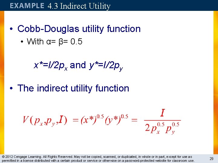
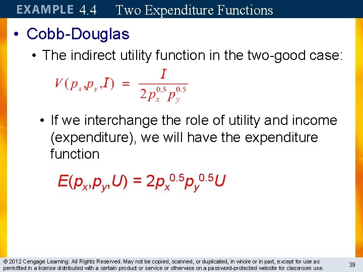
4. 3 Indirect Utility • Cobb-Douglas utility function • With α= β= 0. 5 x*=I/2 px and y*=I/2 py • The indirect utility function © 2012 Cengage Learning. All Rights Reserved. May not be copied, scanned, or duplicated, in whole or in part, except for use as permitted in a license distributed with a certain product or service or otherwise on a password-protected website for classroom use. 29

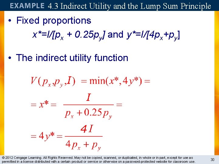
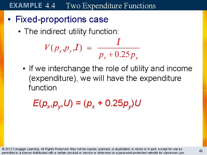
4. 3 Indirect Utility and the Lump Sum Principle • Fixed proportions x*=I/[px + 0. 25 py] and y*=I/[4 px+py] • The indirect utility function I © 2012 Cengage Learning. All Rights Reserved. May not be copied, scanned, or duplicated, in whole or in part, except for use as permitted in a license distributed with a certain product or service or otherwise on a password-protected website for classroom use. 30

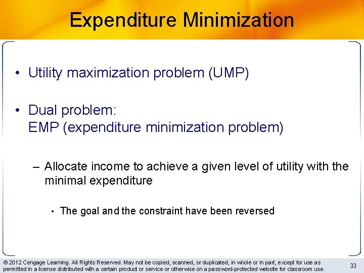
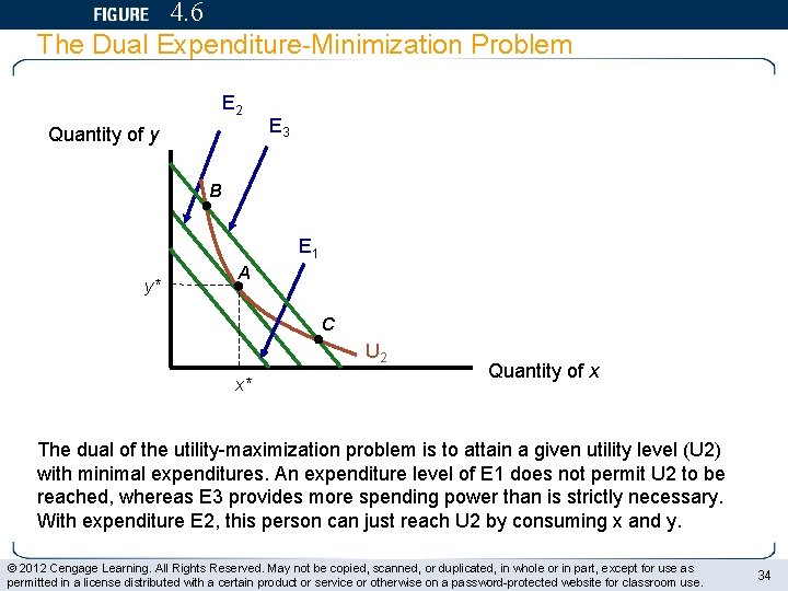
Expenditure Minimization • Utility maximization problem (UMP) • Dual problem: EMP (expenditure minimization problem) – Allocate income to achieve a given level of utility with the minimal expenditure • The goal and the constraint have been reversed © 2012 Cengage Learning. All Rights Reserved. May not be copied, scanned, or duplicated, in whole or in part, except for use as permitted in a license distributed with a certain product or service or otherwise on a password-protected website for classroom use. 33

4. 6 The Dual Expenditure-Minimization Problem E 2 Quantity of y E 3 B E 1 y* A C U 2 x* Quantity of x The dual of the utility-maximization problem is to attain a given utility level (U 2) with minimal expenditures. An expenditure level of E 1 does not permit U 2 to be reached, whereas E 3 provides more spending power than is strictly necessary. With expenditure E 2, this person can just reach U 2 by consuming x and y. © 2012 Cengage Learning. All Rights Reserved. May not be copied, scanned, or duplicated, in whole or in part, except for use as permitted in a license distributed with a certain product or service or otherwise on a password-protected website for classroom use. 34

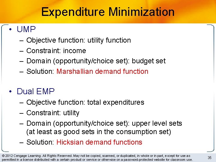
Expenditure Minimization • UMP – – Objective function: utility function Constraint: income Domain (opportunity/choice set): budget set Solution: Marshallian demand function • Dual EMP – Objective function: total expenditures – Constraint: utility – Domain (opportunity/choice set): upper level sets (at least as good sets in the consumption set) – Solution: Hicksian demand functions © 2012 Cengage Learning. All Rights Reserved. May not be copied, scanned, or duplicated, in whole or in part, except for use as permitted in a license distributed with a certain product or service or otherwise on a password-protected website for classroom use. 35

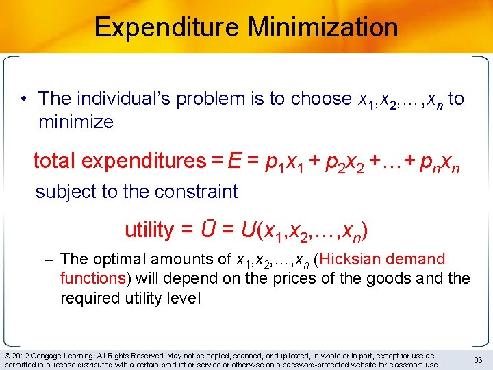
Expenditure Minimization • The individual’s problem is to choose x 1, x 2, …, xn to minimize total expenditures = E = p 1 x 1 + p 2 x 2 +…+ pnxn subject to the constraint utility = Ū = U(x 1, x 2, …, xn) – The optimal amounts of x 1, x 2, …, xn (Hicksian demand functions) will depend on the prices of the goods and the required utility level © 2012 Cengage Learning. All Rights Reserved. May not be copied, scanned, or duplicated, in whole or in part, except for use as permitted in a license distributed with a certain product or service or otherwise on a password-protected website for classroom use. 36

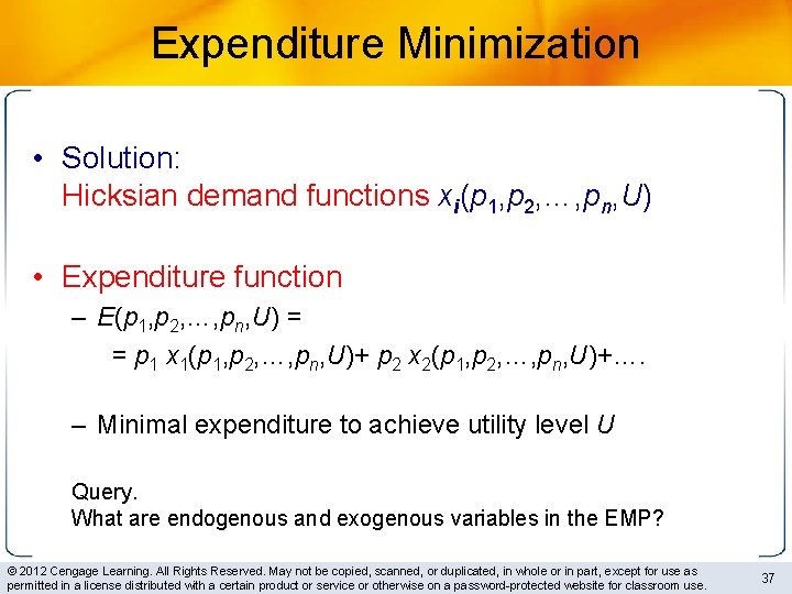
Expenditure Minimization • Solution: Hicksian demand functions xi(p 1, p 2, …, pn, U) • Expenditure function – E(p 1, p 2, …, pn, U) = = p 1 x 1(p 1, p 2, …, pn, U)+ p 2 x 2(p 1, p 2, …, pn, U)+…. – Minimal expenditure to achieve utility level U Query. What are endogenous and exogenous variables in the EMP? © 2012 Cengage Learning. All Rights Reserved. May not be copied, scanned, or duplicated, in whole or in part, except for use as permitted in a license distributed with a certain product or service or otherwise on a password-protected website for classroom use. 37

Expenditure Minimization • The expenditure function and the indirect utility function – Are inversely related – Both depend on market prices – But involve different constraints • Query. Identify the constraints of the UMP and EMP respectively. © 2012 Cengage Learning. All Rights Reserved. May not be copied, scanned, or duplicated, in whole or in part, except for use as permitted in a license distributed with a certain product or service or otherwise on a password-protected website for classroom use. 38

4. 4 Two Expenditure Functions • Cobb-Douglas • The indirect utility function in the two-good case: • If we interchange the role of utility and income (expenditure), we will have the expenditure function E(px, py, U) = 2 px 0. 5 py 0. 5 U © 2012 Cengage Learning. All Rights Reserved. May not be copied, scanned, or duplicated, in whole or in part, except for use as permitted in a license distributed with a certain product or service or otherwise on a password-protected website for classroom use. 39

4. 4 Two Expenditure Functions • Fixed-proportions case • The indirect utility function: • If we interchange the role of utility and income (expenditure), we will have the expenditure function E(px, py, U) = (px + 0. 25 py)U © 2012 Cengage Learning. All Rights Reserved. May not be copied, scanned, or duplicated, in whole or in part, except for use as permitted in a license distributed with a certain product or service or otherwise on a password-protected website for classroom use. 40

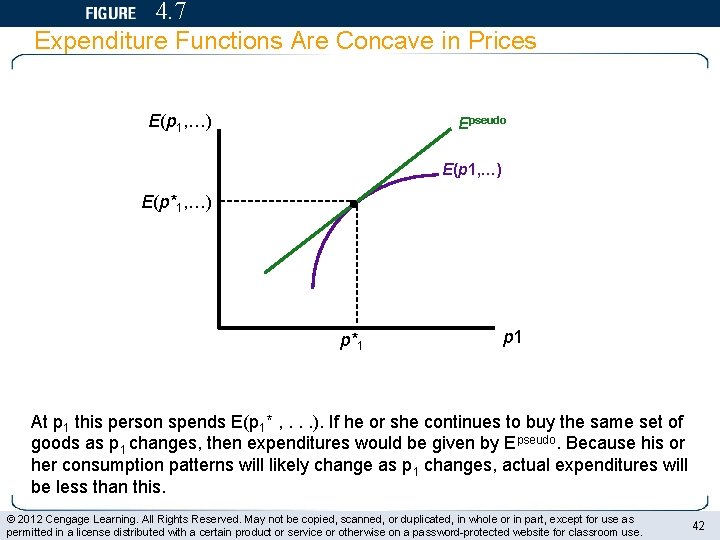
Properties of Expenditure Functions • Homogeneity – A doubling of all prices will precisely double the value of required expenditures • Homogeneous of degree one in prices • Nondecreasing in prices – ∂E/∂pi ≥ 0 for every good • Concave in prices – Functions that always lie below tangents to them © 2012 Cengage Learning. All Rights Reserved. May not be copied, scanned, or duplicated, in whole or in part, except for use as permitted in a license distributed with a certain product or service or otherwise on a password-protected website for classroom use. 41

4. 7 Expenditure Functions Are Concave in Prices E(p 1, …) Epseudo E(p 1, …) E(p*1, …) p*1 p 1 At p 1 this person spends E(p 1* , . . . ). If he or she continues to buy the same set of goods as p 1 changes, then expenditures would be given by Epseudo. Because his or her consumption patterns will likely change as p 1 changes, actual expenditures will be less than this. © 2012 Cengage Learning. All Rights Reserved. May not be copied, scanned, or duplicated, in whole or in part, except for use as permitted in a license distributed with a certain product or service or otherwise on a password-protected website for classroom use. 42

EMP and UMP • Solutions to the UMP and the EMP – Marshallian demand functions xi(p 1, p 2, …, pn, I) – Hicksian demand functions xi(p 1, p 2, …, pn, U) – – Query. What exactly do Hicksian demand functions identify? What exactly do Marshallien demand functions identify? Relate xi(p 1, p 2, …, pn, U) to xi(p 1, p 2, …, pn, I) © 2012 Cengage Learning. All Rights Reserved. May not be copied, scanned, or duplicated, in whole or in part, except for use as permitted in a license distributed with a certain product or service or otherwise on a password-protected website for classroom use. 43