Chapter 4 UTILITY MAXIMIZATION AND CHOICE Copyright 2005

Chapter 4 UTILITY MAXIMIZATION AND CHOICE Copyright © 2005 by South-Western, a division of Thomson Learning. All rights reserved. 1

Complaints about the Economic Approach • No real individuals make the kinds of “lightning calculations” required for utility maximization • The utility-maximization model predicts many aspects of behavior • Thus, economists assume that people behave as if they made such calculations 2

Complaints about the Economic Approach • The economic model of choice is extremely selfish because no one has solely self-centered goals • Nothing in the utility-maximization model prevents individuals from deriving satisfaction from “doing good” 3

Optimization Principle • To maximize utility, given a fixed amount of income to spend, an individual will buy the goods and services: – that exhaust his or her total income – for which the psychic rate of trade-off between any goods (the MRS) is equal to the rate at which goods can be traded for one another in the marketplace 4

A Numerical Illustration • Assume that the individual’s MRS = 1 – willing to trade one unit of x for one unit of y • Suppose the price of x = $2 and the price of y = $1 • The individual can be made better off – trade 1 unit of x for 2 units of y in the marketplace 5

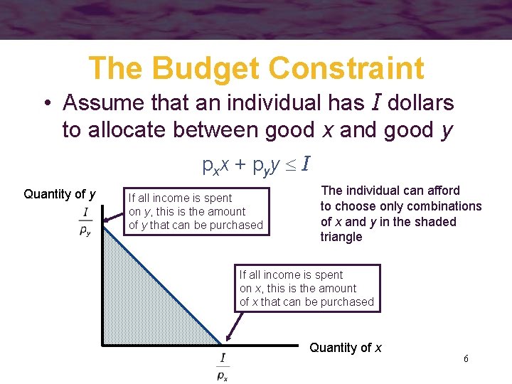
The Budget Constraint • Assume that an individual has I dollars to allocate between good x and good y pxx + pyy I Quantity of y If all income is spent on y, this is the amount of y that can be purchased The individual can afford to choose only combinations of x and y in the shaded triangle If all income is spent on x, this is the amount of x that can be purchased Quantity of x 6

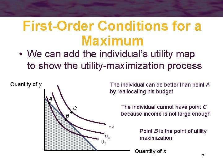
First-Order Conditions for a Maximum • We can add the individual’s utility map to show the utility-maximization process Quantity of y The individual can do better than point A by reallocating his budget A The individual cannot have point C because income is not large enough C B U 3 U 2 U 1 Point B is the point of utility maximization Quantity of x 7

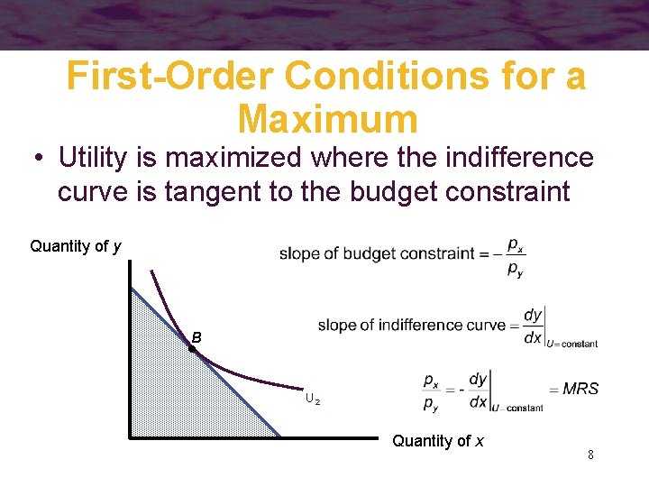
First-Order Conditions for a Maximum • Utility is maximized where the indifference curve is tangent to the budget constraint Quantity of y B U 2 Quantity of x 8

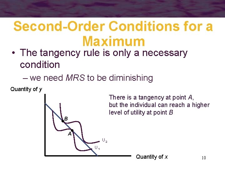
Second-Order Conditions for a Maximum • The tangency rule is only necessary but not sufficient unless we assume that MRS is diminishing – if MRS is diminishing, then indifference curves are strictly convex • If MRS is not diminishing, then we must check second-order conditions to ensure that we are at a maximum 9

Second-Order Conditions for a Maximum • The tangency rule is only a necessary condition – we need MRS to be diminishing Quantity of y There is a tangency at point A, but the individual can reach a higher level of utility at point B B A U 2 U 1 Quantity of x 10

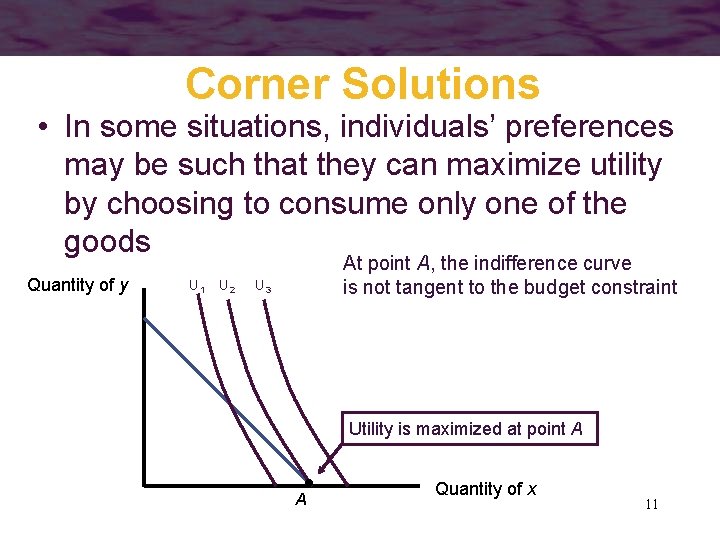
Corner Solutions • In some situations, individuals’ preferences may be such that they can maximize utility by choosing to consume only one of the goods Quantity of y U 1 U 2 At point A, the indifference curve is not tangent to the budget constraint U 3 Utility is maximized at point A A Quantity of x 11

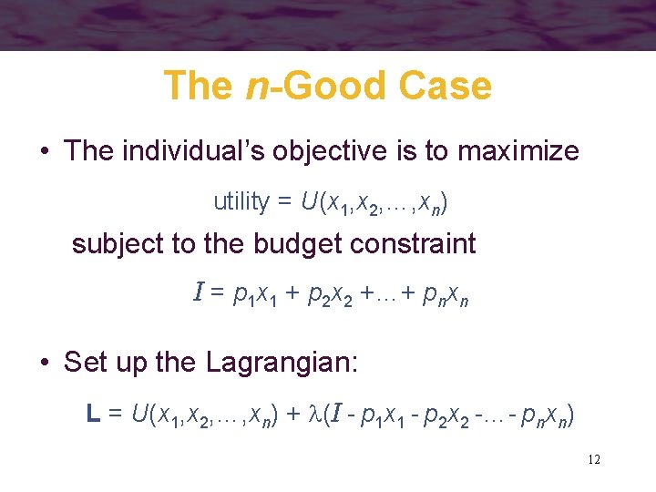
The n-Good Case • The individual’s objective is to maximize utility = U(x 1, x 2, …, xn) subject to the budget constraint I = p 1 x 1 + p 2 x 2 +…+ pnxn • Set up the Lagrangian: L = U(x 1, x 2, …, xn) + (I - p 1 x 1 - p 2 x 2 -…- pnxn) 12

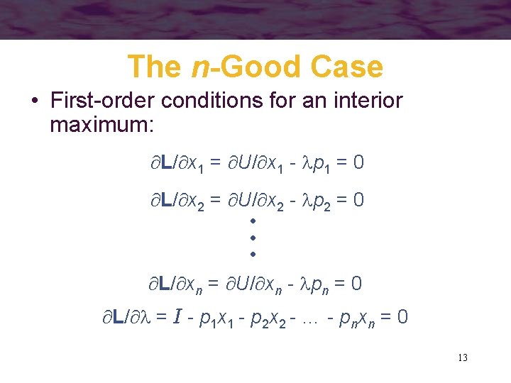
The n-Good Case • First-order conditions for an interior maximum: L/ x 1 = U/ x 1 - p 1 = 0 L/ x 2 = U/ x 2 - p 2 = 0 • • • L/ xn = U/ xn - pn = 0 L/ = I - p 1 x 1 - p 2 x 2 - … - pnxn = 0 13

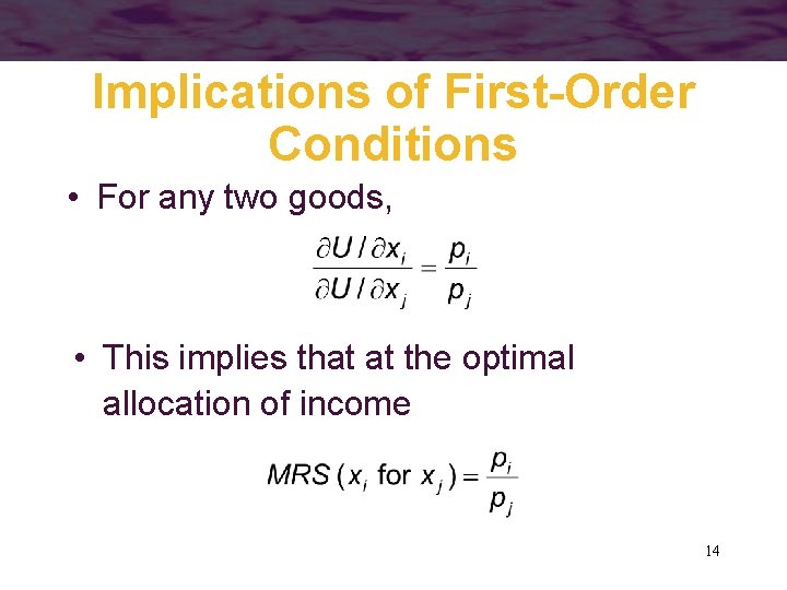
Implications of First-Order Conditions • For any two goods, • This implies that at the optimal allocation of income 14

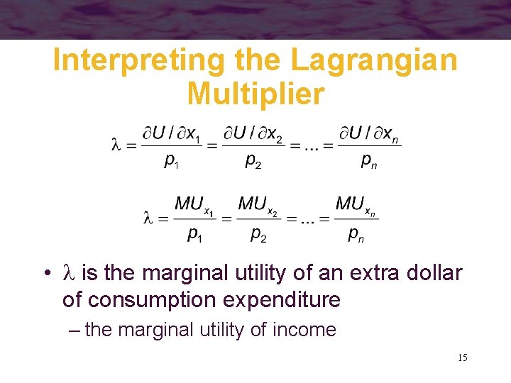
Interpreting the Lagrangian Multiplier • is the marginal utility of an extra dollar of consumption expenditure – the marginal utility of income 15

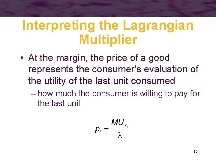
Interpreting the Lagrangian Multiplier • At the margin, the price of a good represents the consumer’s evaluation of the utility of the last unit consumed – how much the consumer is willing to pay for the last unit 16

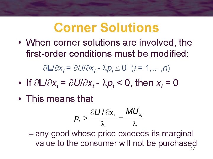
Corner Solutions • When corner solutions are involved, the first-order conditions must be modified: L/ xi = U/ xi - pi 0 (i = 1, …, n) • If L/ xi = U/ xi - pi < 0, then xi = 0 • This means that – any good whose price exceeds its marginal value to the consumer will not be purchased 17

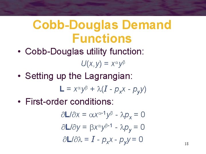
Cobb-Douglas Demand Functions • Cobb-Douglas utility function: U(x, y) = x y • Setting up the Lagrangian: L = x y + (I - pxx - pyy) • First-order conditions: L/ x = x -1 y - px = 0 L/ y = x y -1 - py = 0 L/ = I - pxx - pyy = 0 18

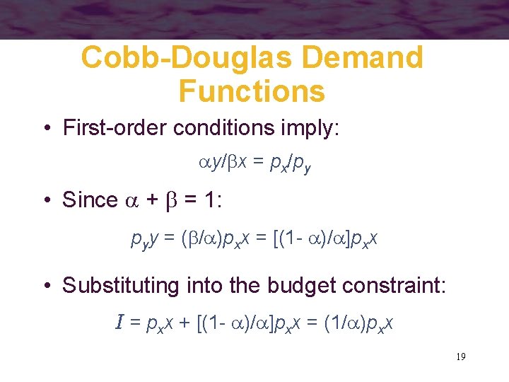
Cobb-Douglas Demand Functions • First-order conditions imply: y/ x = px/py • Since + = 1: pyy = ( / )pxx = [(1 - )/ ]pxx • Substituting into the budget constraint: I = pxx + [(1 - )/ ]pxx = (1/ )pxx 19

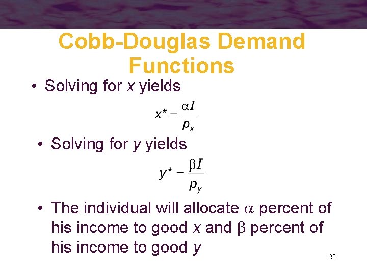
Cobb-Douglas Demand Functions • Solving for x yields • Solving for y yields • The individual will allocate percent of his income to good x and percent of his income to good y 20

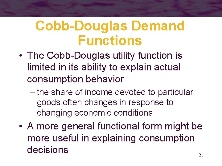
Cobb-Douglas Demand Functions • The Cobb-Douglas utility function is limited in its ability to explain actual consumption behavior – the share of income devoted to particular goods often changes in response to changing economic conditions • A more general functional form might be more useful in explaining consumption decisions 21

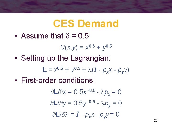
CES Demand • Assume that = 0. 5 U(x, y) = x 0. 5 + y 0. 5 • Setting up the Lagrangian: L = x 0. 5 + y 0. 5 + (I - pxx - pyy) • First-order conditions: L/ x = 0. 5 x -0. 5 - px = 0 L/ y = 0. 5 y -0. 5 - py = 0 L/ = I - pxx - pyy = 0 22

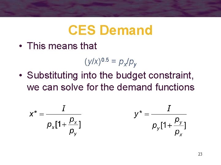
CES Demand • This means that (y/x)0. 5 = px/py • Substituting into the budget constraint, we can solve for the demand functions 23

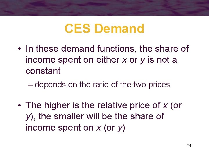
CES Demand • In these demand functions, the share of income spent on either x or y is not a constant – depends on the ratio of the two prices • The higher is the relative price of x (or y), the smaller will be the share of income spent on x (or y) 24

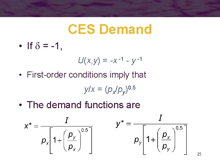
CES Demand • If = -1, U(x, y) = -x -1 - y -1 • First-order conditions imply that y/x = (px/py)0. 5 • The demand functions are 25

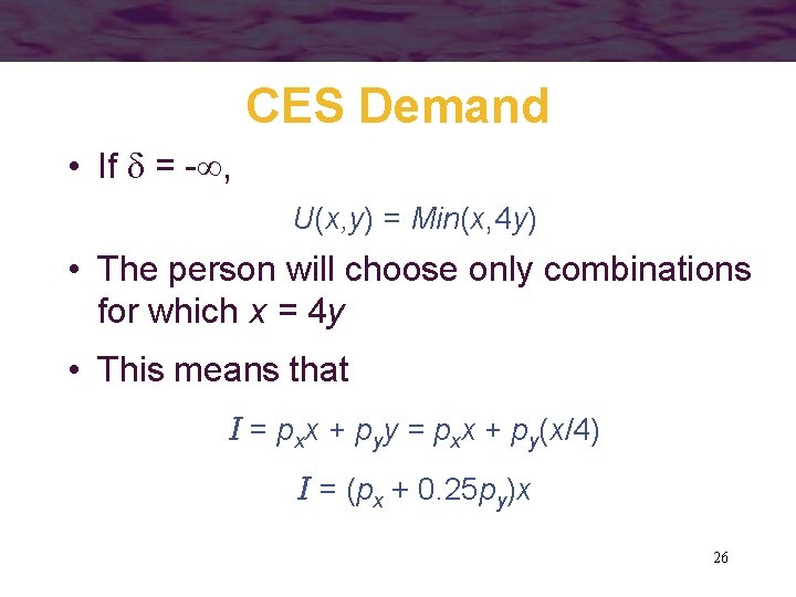
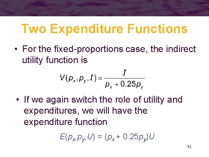
CES Demand • If = - , U(x, y) = Min(x, 4 y) • The person will choose only combinations for which x = 4 y • This means that I = pxx + pyy = pxx + py(x/4) I = (px + 0. 25 py)x 26

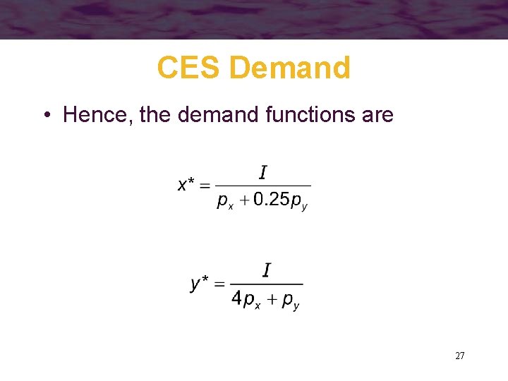
CES Demand • Hence, the demand functions are 27

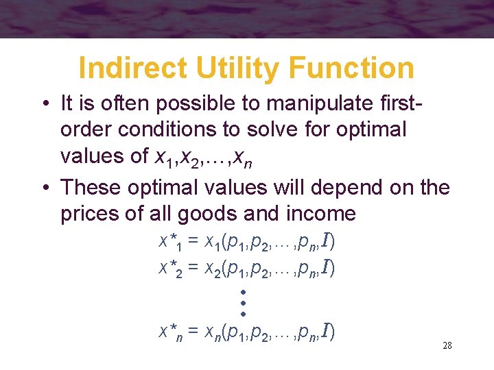
Indirect Utility Function • It is often possible to manipulate firstorder conditions to solve for optimal values of x 1, x 2, …, xn • These optimal values will depend on the prices of all goods and income x*1 = x 1(p 1, p 2, …, pn, I) x*2 = x 2(p 1, p 2, …, pn, I) • • • x*n = xn(p 1, p 2, …, pn, I) 28

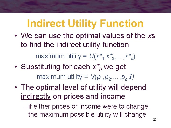
Indirect Utility Function • We can use the optimal values of the xs to find the indirect utility function maximum utility = U(x*1, x*2, …, x*n) • Substituting for each x*i, we get maximum utility = V(p 1, p 2, …, pn, I) • The optimal level of utility will depend indirectly on prices and income – if either prices or income were to change, the maximum possible utility will change 29

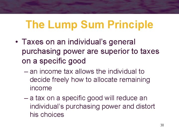
The Lump Sum Principle • Taxes on an individual’s general purchasing power are superior to taxes on a specific good – an income tax allows the individual to decide freely how to allocate remaining income – a tax on a specific good will reduce an individual’s purchasing power and distort his choices 30

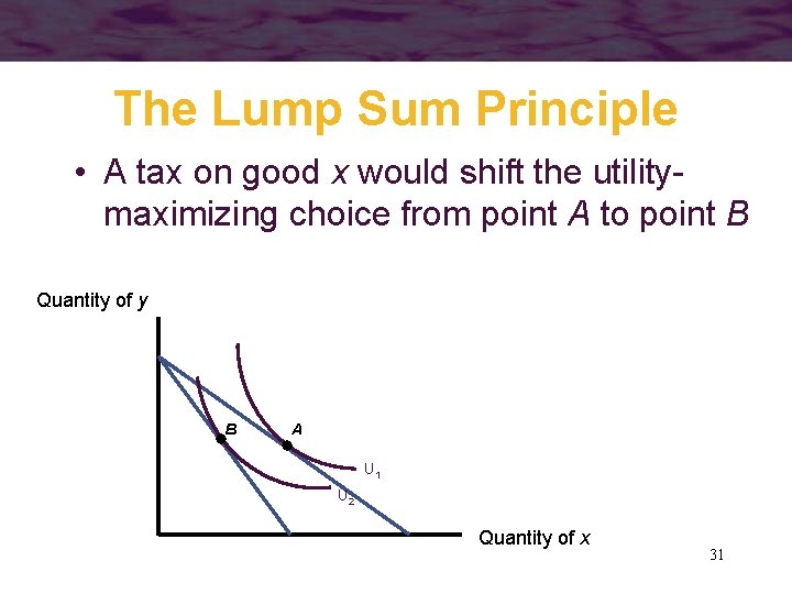
The Lump Sum Principle • A tax on good x would shift the utilitymaximizing choice from point A to point B Quantity of y B A U 1 U 2 Quantity of x 31

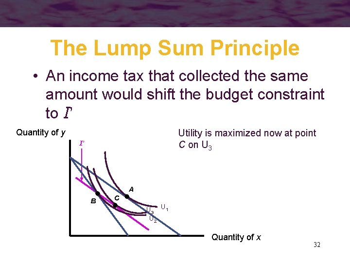
The Lump Sum Principle • An income tax that collected the same amount would shift the budget constraint to I’ Quantity of y Utility is maximized now at point C on U 3 I’ A B C U 3 U 1 U 2 Quantity of x 32

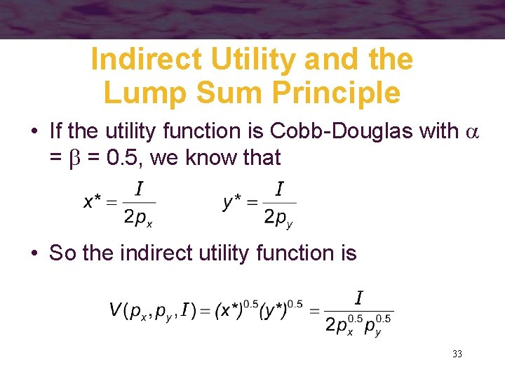
Indirect Utility and the Lump Sum Principle • If the utility function is Cobb-Douglas with = = 0. 5, we know that • So the indirect utility function is 33

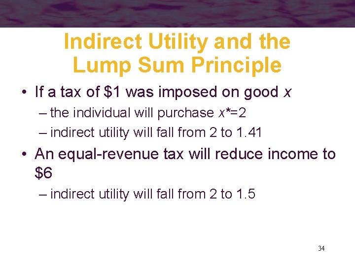
Indirect Utility and the Lump Sum Principle • If a tax of $1 was imposed on good x – the individual will purchase x*=2 – indirect utility will fall from 2 to 1. 41 • An equal-revenue tax will reduce income to $6 – indirect utility will fall from 2 to 1. 5 34

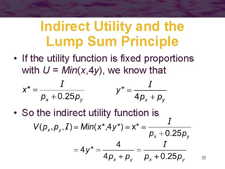
Indirect Utility and the Lump Sum Principle • If the utility function is fixed proportions with U = Min(x, 4 y), we know that • So the indirect utility function is 35

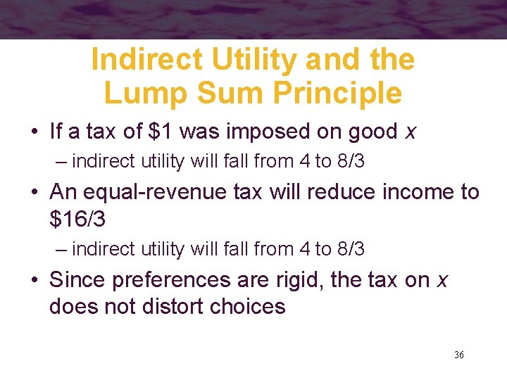
Indirect Utility and the Lump Sum Principle • If a tax of $1 was imposed on good x – indirect utility will fall from 4 to 8/3 • An equal-revenue tax will reduce income to $16/3 – indirect utility will fall from 4 to 8/3 • Since preferences are rigid, the tax on x does not distort choices 36

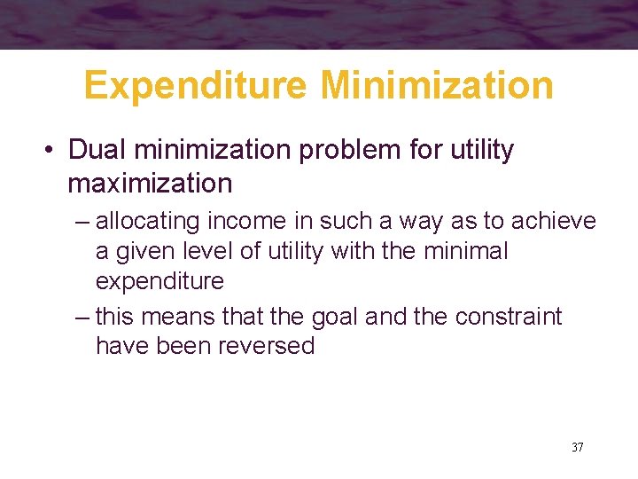
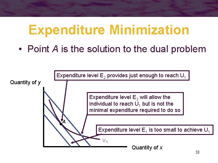
Expenditure Minimization • Dual minimization problem for utility maximization – allocating income in such a way as to achieve a given level of utility with the minimal expenditure – this means that the goal and the constraint have been reversed 37

Expenditure Minimization • Point A is the solution to the dual problem Quantity of y Expenditure level E 2 provides just enough to reach U 1 Expenditure level E 3 will allow the individual to reach U 1 but is not the minimal expenditure required to do so A Expenditure level E 1 is too small to achieve U 1 Quantity of x 38

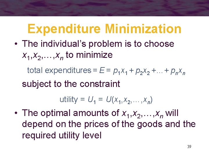
Expenditure Minimization • The individual’s problem is to choose x 1, x 2, …, xn to minimize total expenditures = E = p 1 x 1 + p 2 x 2 +…+ pnxn subject to the constraint utility = U 1 = U(x 1, x 2, …, xn) • The optimal amounts of x 1, x 2, …, xn will depend on the prices of the goods and the required utility level 39

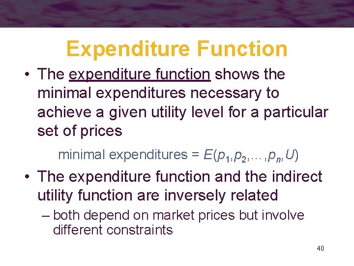
Expenditure Function • The expenditure function shows the minimal expenditures necessary to achieve a given utility level for a particular set of prices minimal expenditures = E(p 1, p 2, …, pn, U) • The expenditure function and the indirect utility function are inversely related – both depend on market prices but involve different constraints 40

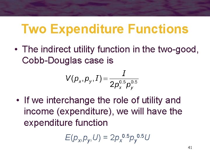
Two Expenditure Functions • The indirect utility function in the two-good, Cobb-Douglas case is • If we interchange the role of utility and income (expenditure), we will have the expenditure function E(px, py, U) = 2 px 0. 5 py 0. 5 U 41

Two Expenditure Functions • For the fixed-proportions case, the indirect utility function is • If we again switch the role of utility and expenditures, we will have the expenditure function E(px, py, U) = (px + 0. 25 py)U 42

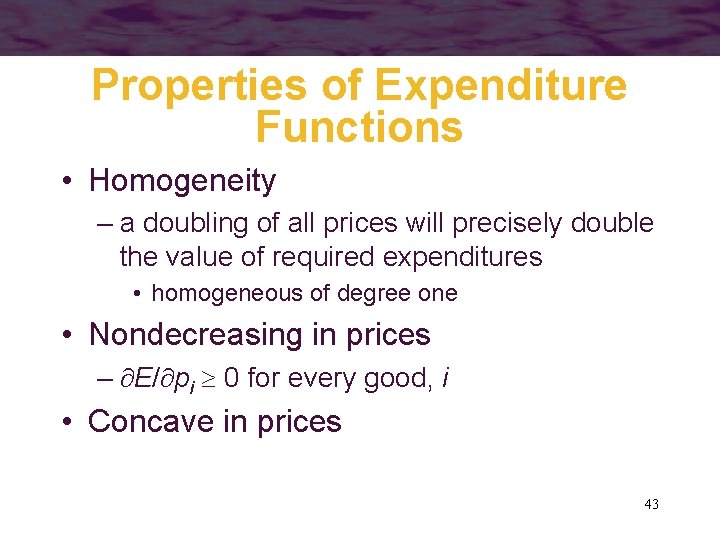
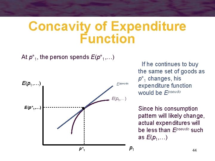
Properties of Expenditure Functions • Homogeneity – a doubling of all prices will precisely double the value of required expenditures • homogeneous of degree one • Nondecreasing in prices – E/ pi 0 for every good, i • Concave in prices 43

Concavity of Expenditure Function At p*1, the person spends E(p*1, …) E(p 1, …) If he continues to buy the same set of goods as p*1 changes, his expenditure function would be Epseudo E(p 1, …) E(p*1, …) Since his consumption pattern will likely change, actual expenditures will be less than Epseudo such as E(p 1, …) p*1 p 1 44

Important Points to Note: • To reach a constrained maximum, an individual should: – spend all available income – choose a commodity bundle such that the MRS between any two goods is equal to the ratio of the goods’ prices • the individual will equate the ratios of the marginal utility to price for every good that is actually consumed 45

Important Points to Note: • Tangency conditions are only firstorder conditions – the individual’s indifference map must exhibit diminishing MRS – the utility function must be strictly quasiconcave 46

Important Points to Note: • Tangency conditions must also be modified to allow for corner solutions – the ratio of marginal utility to price will be below the common marginal benefitmarginal cost ratio for goods actually bought 47

Important Points to Note: • The individual’s optimal choices implicitly depend on the parameters of his budget constraint – choices observed will be implicit functions of prices and income – utility will also be an indirect function of prices and income 48

Important Points to Note: • The dual problem to the constrained utility-maximization problem is to minimize the expenditure required to reach a given utility target – yields the same optimal solution as the primary problem – leads to expenditure functions in which spending is a function of the utility target and prices 49