Using Multiples for Valuation Why Use Multiples A

Using Multiples for Valuation

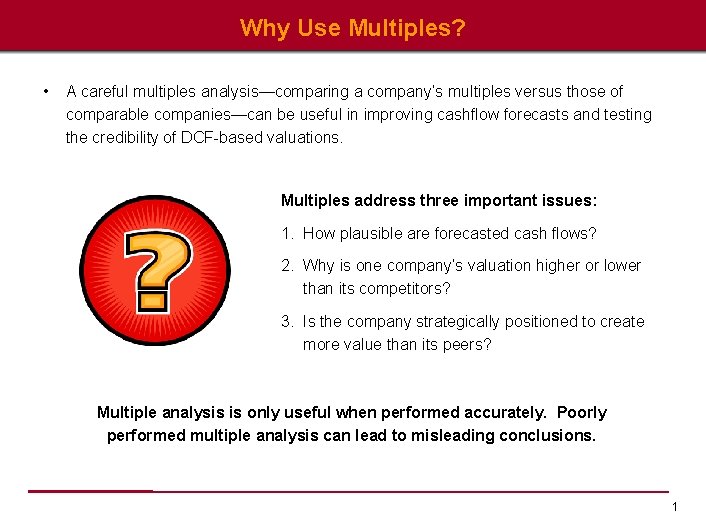
Why Use Multiples? • A careful multiples analysis—comparing a company’s multiples versus those of comparable companies—can be useful in improving cashflow forecasts and testing the credibility of DCF-based valuations. Multiples address three important issues: 1. How plausible are forecasted cash flows? 2. Why is one company’s valuation higher or lower than its competitors? 3. Is the company strategically positioned to create more value than its peers? Multiple analysis is only useful when performed accurately. Poorly performed multiple analysis can lead to misleading conclusions. 1

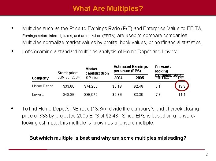
What Are Multiples? • Multiples such as the Price-to-Earnings Ratio (P/E) and Enterprise-Value-to-EBITA, Earnings before interest, taxes, and amortization (EBITA), are used to compare companies. Multiples normalize market values by profits, book values, or nonfinancial statistics. • Let’s examine a standard multiples analysis of Home Depot and Lowes: Company • Stock price July 23, 2004 Market capitalization $ Million Estimated Earnings per share (EPS) 2004 2005 Forwardlooking multiples, 2004 EBITDA P/E Home Depot $33. 00 $74, 250 $2. 18 $2. 48 7. 1 13. 3 Lowe’s $48. 39 $39, 075 $2. 86 $3. 36 7. 3 14. 4 To find Home Depot’s P/E ratio (13. 3 x), divide the company’s end of week closing price of $33 by projected 2005 EPS of $2. 48. Since EPS is based on a forwardlooking estimate, this multiple is known as a forward multiple. But which multiple is best and why are some multiples misleading? 2

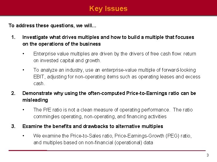
Key Issues To address these questions, we will… 1. 2. Investigate what drives multiples and how to build a multiple that focuses on the operations of the business • Enterprise value multiples are driven by the drivers of free cash flow: return on invested capital and growth. • To analyze an industry, use an enterprise-value multiple of forward-looking EBIT, adjusting for non-operating items such as operating leases and excess cash. Demonstrate why using the often-computed Price-to-Earnings ratio can be misleading • 3. The P/E ratio is not a clean measure of operating performance. The ratio commingles operating, non-operating, and financing activities Examine the benefits and drawbacks to alternative multiples • We examine the Price-to-Sales ratio, Price-Earnings-Growth (PEG) ratio, and multiples based on non-financial (operational) data 3

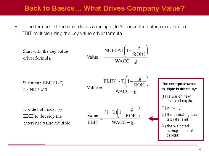
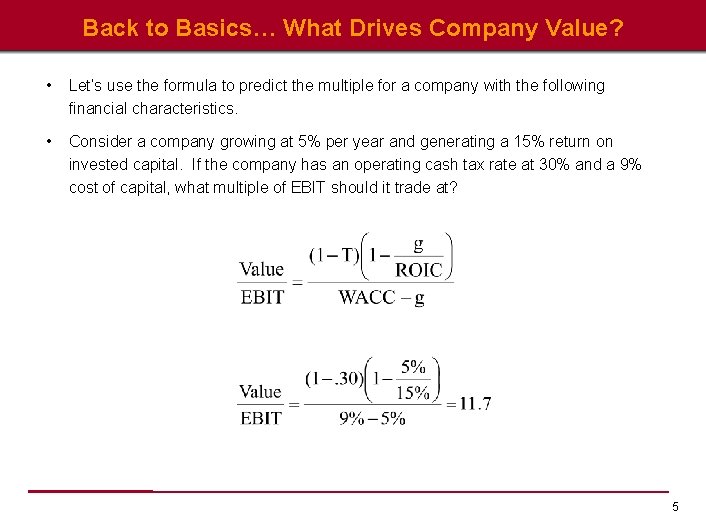
Back to Basics… What Drives Company Value? • To better understand what drives a multiple, let’s derive the enterprise value to EBIT multiple using the key value driver formula. Start with the key value driver formula. Substitute EBIT(1 -T) for NOPLAT The enterprise value multiple is driven by: (1) return on new invested capital, Divide both sides by EBIT to develop the enterprise value multiple. (2) growth, (3) the operating cash tax rate, and (4) the weighted average cost of capital 4

Back to Basics… What Drives Company Value? • Let’s use the formula to predict the multiple for a company with the following financial characteristics. • Consider a company growing at 5% per year and generating a 15% return on invested capital. If the company has an operating cash tax rate at 30% and a 9% cost of capital, what multiple of EBIT should it trade at? 5

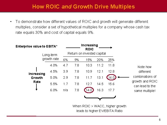
How ROIC and Growth Drive Multiples • To demonstrate how different values of ROIC and growth will generate different multiples, consider a set of hypothetical multiples for a company whose cash tax rate equals 30% and cost of capital equals 9%. Enterprise value to EBITA* Long-term growth rate Increasing Growth Rate Increasing ROIC Return on invested capital 6% 9% 15% 20% 25% 4. 0% 4. 7 7. 8 10. 3 11. 2 11. 8 4. 5% 3. 9 7. 8 10. 9 12. 1 12. 8 5. 0% 2. 9 7. 8 11. 7 13. 1 14. 0 5. 5% 1. 7 7. 8 12. 7 14. 5 15. 6 6. 0% n/a 7. 8 14. 0 16. 3 17. 7 Note how different combinations of growth and ROIC can lead to the same multiple! When ROIC > WACC, higher growth leads to higher EV/EBITA Ratio 6

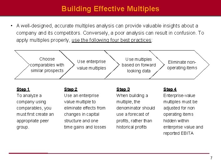
Building Effective Multiples • A well-designed, accurate multiples analysis can provide valuable insights about a company and its competitors. Conversely, a poor analysis can result in confusion. To apply multiples properly, use the following four best practices: Choose comparables with similar prospects Step 1 To analyze a company using comparables, you must first create an appropriate peer group. Use enterprise value multiples Use multiples based on forward looking data Step 2 Use an enterprise value multiple to eliminate effects from changes in capital structure and one time gains and losses Step 3 When building a multiple, the denominator should use a forecast of profits, rather than historical profits Eliminate nonoperating items Step 4 Enterprise-value multiples must be adjusted for non operating items hidden within enterprise value and reported EBITA 7

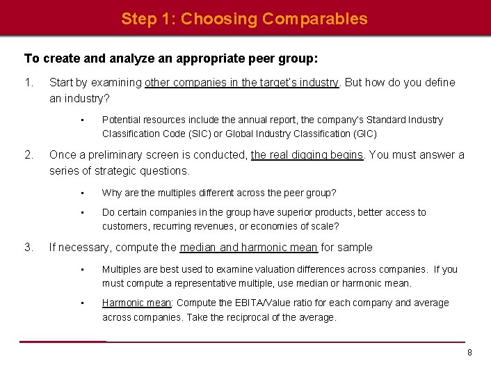
Step 1: Choosing Comparables To create and analyze an appropriate peer group: 1. Start by examining other companies in the target’s industry. But how do you define an industry? • 2. 3. Potential resources include the annual report, the company’s Standard Industry Classification Code (SIC) or Global Industry Classification (GIC) Once a preliminary screen is conducted, the real digging begins. You must answer a series of strategic questions. • Why are the multiples different across the peer group? • Do certain companies in the group have superior products, better access to customers, recurring revenues, or economies of scale? If necessary, compute the median and harmonic mean for sample • Multiples are best used to examine valuation differences across companies. If you must compute a representative multiple, use median or harmonic mean. • Harmonic mean: Compute the EBITA/Value ratio for each company and average across companies. Take the reciprocal of the average. 8

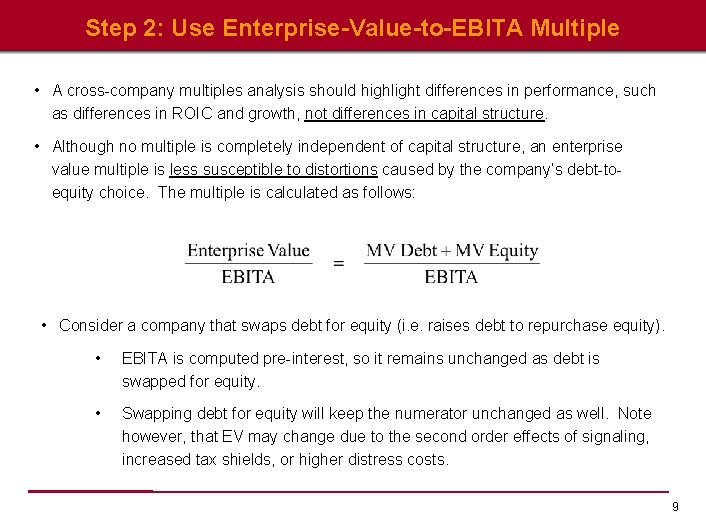
Step 2: Use Enterprise-Value-to-EBITA Multiple • A cross-company multiples analysis should highlight differences in performance, such as differences in ROIC and growth, not differences in capital structure. • Although no multiple is completely independent of capital structure, an enterprise value multiple is less susceptible to distortions caused by the company’s debt-toequity choice. The multiple is calculated as follows: • Consider a company that swaps debt for equity (i. e. raises debt to repurchase equity). • EBITA is computed pre-interest, so it remains unchanged as debt is swapped for equity. • Swapping debt for equity will keep the numerator unchanged as well. Note however, that EV may change due to the second order effects of signaling, increased tax shields, or higher distress costs. 9

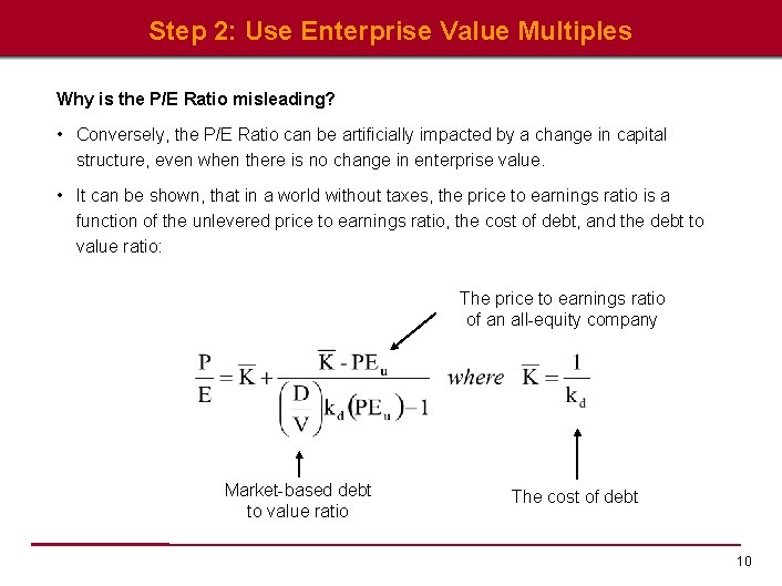
Step 2: Use Enterprise Value Multiples Why is the P/E Ratio misleading? • Conversely, the P/E Ratio can be artificially impacted by a change in capital structure, even when there is no change in enterprise value. • It can be shown, that in a world without taxes, the price to earnings ratio is a function of the unlevered price to earnings ratio, the cost of debt, and the debt to value ratio: The price to earnings ratio of an all-equity company Market-based debt to value ratio The cost of debt 10

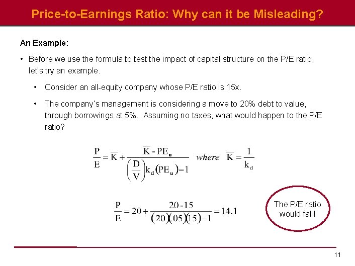
Price-to-Earnings Ratio: Why can it be Misleading? An Example: • Before we use the formula to test the impact of capital structure on the P/E ratio, let’s try an example. • Consider an all-equity company whose P/E ratio is 15 x. • The company’s management is considering a move to 20% debt to value, through borrowings at 5%. Assuming no taxes, what would happen to the P/E ratio? The P/E ratio would fall! 11

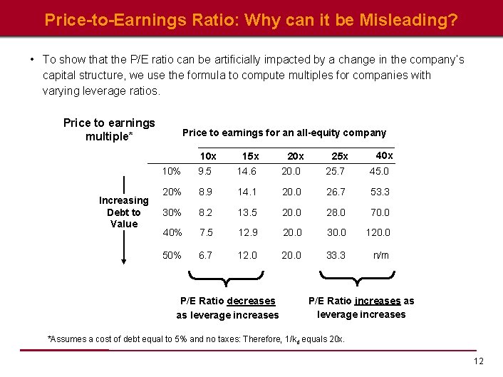
Price-to-Earnings Ratio: Why can it be Misleading? • To show that the P/E ratio can be artificially impacted by a change in the company’s capital structure, we use the formula to compute multiples for companies with varying leverage ratios. Price to earnings multiple* Price to earnings for an all-equity company 10 x Increasing Debt to Value 15 x 20 x 25 x 40 x 10% 9. 5 14. 6 20. 0 25. 7 45. 0 20% 8. 9 14. 1 20. 0 26. 7 53. 3 30% 8. 2 13. 5 20. 0 28. 0 70. 0 40% 7. 5 12. 9 20. 0 30. 0 120. 0 50% 6. 7 12. 0 20. 0 33. 3 n/m P/E Ratio decreases as leverage increases P/E Ratio increases as leverage increases *Assumes a cost of debt equal to 5% and no taxes: Therefore, 1/kd equals 20 x. 12

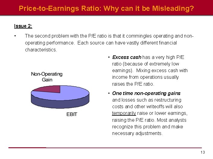
Price-to-Earnings Ratio: Why can it be Misleading? Issue 2: • The second problem with the P/E ratio is that it commingles operating and nonoperating performance. Each source can have vastly different financial characteristics. • Excess cash has a very high P/E ratio (because of extremely low earnings). Mixing excess cash with income from operations usually raises the P/E ratio. • One time non-operating gains and losses such as restructuring costs and other writeoffs will also temporarily raise or lower earnings, raising the P/E ratio. Most analysts recognize this problem and make necessary adjustments. 13

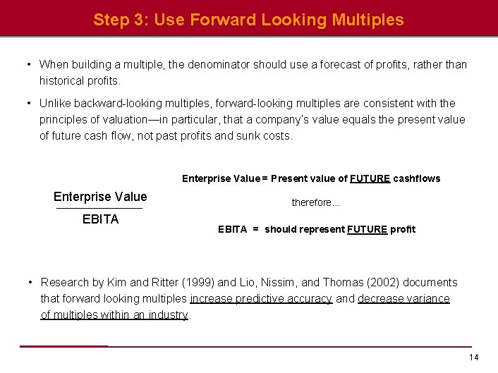
Step 3: Use Forward Looking Multiples • When building a multiple, the denominator should use a forecast of profits, rather than historical profits. • Unlike backward-looking multiples, forward-looking multiples are consistent with the principles of valuation—in particular, that a company’s value equals the present value of future cash flow, not past profits and sunk costs. Enterprise Value = Present value of FUTURE cashflows Enterprise Value EBITA therefore… EBITA = should represent FUTURE profit • Research by Kim and Ritter (1999) and Lio, Nissim, and Thomas (2002) documents that forward looking multiples increase predictive accuracy and decrease variance of multiples within an industry. 14

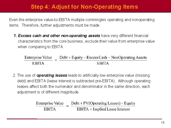
Step 4: Adjust for Non-Operating Items Even the enterprise value-to-EBITA multiple commingles operating and nonoperating items. Therefore, further adjustments must be made. 1. Excess cash and other non-operating assets have very different financial characteristics from the core business, exclude their value from enterprise value when comparing to EBITA. 2. The use of operating leases leads to artificially low enterprise value (missing debt) and EBITA (lease interest is subtracted pre-EBITA). Although operating leases affect both the numerator and denominator in the same direction, each adjustment is of different magnitude. 15

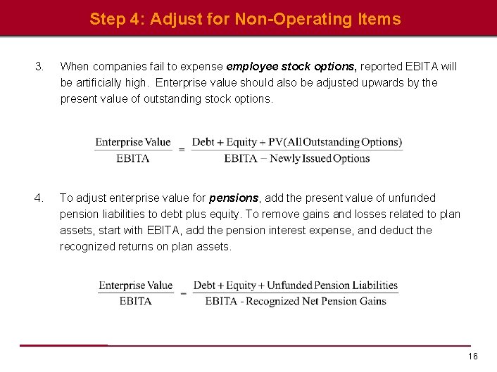
Step 4: Adjust for Non-Operating Items 3. When companies fail to expense employee stock options, reported EBITA will be artificially high. Enterprise value should also be adjusted upwards by the present value of outstanding stock options. 4. To adjust enterprise value for pensions, add the present value of unfunded pension liabilities to debt plus equity. To remove gains and losses related to plan assets, start with EBITA, add the pension interest expense, and deduct the recognized returns on plan assets. 16

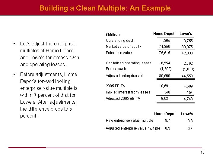
Building a Clean Multiple: An Example $ Million • • Let’s adjust the enterprise multiples of Home Depot and Lowe’s for excess cash and operating leases. Before adjustments, Home Depot’s forward looking enterprise-value multiple is within 7 percent of that for Lowe’s. After adjustments, the difference drops to 5 percent. Home Depot Outstanding debt Lowe’s 1, 365 3, 755 Market value of equity 74, 250 39, 075 Enterprise value 75, 615 42, 830 Capitalized operating leases 6, 554 2, 762 Excess cash (1, 609) (1, 033) Adjusted enterprise value 80, 560 44, 559 8, 691 4, 589 340 154 9, 031 4, 743 Home Depot Lowe’s 2005 EBITA Implied interest from leases Adjusted 2005 EBITA Raw enterprise value multiple 8. 7 9. 3 Adjusted enterprise value multiple 8. 9 9. 4 17

An Examination of Alternative Multiples Although we have so far focused on enterprise-value multiples based on EBITA , other multiples can prove helpful in certain situations. • Price-to-Sales Multiple. An enterprise-value-to-sales multiple imposes an additional important restriction beyond the EV/EBITA multiple: similar operating margins on the company’s existing business. For most industries, this restriction is overly burdensome. • Price Earnings Growth (PEG) Ratio. Whereas a price-to-sales ratio further restricts the enterprise-to-EBITA multiple, the PEG ratio is more flexible than the enterprise multiple, because it allows expected growth to vary across companies. • EV/EBITDA vs. EV/EBIT multiples. EBITDA is popular because the statistic is closer to cashflow than EBIT, but fails to measure reinvestment, or capture differences in equipment outsourcing. • Multiples of operational data. When financial data is sparse, compute nonfinancial multiples, which compare enterprise value to one or more operating statistics, such as Web site hits, unique visitors, or number of subscribers. 18

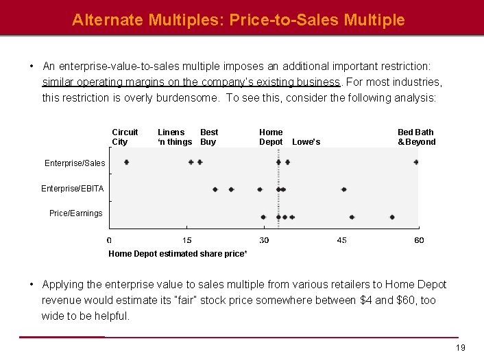
Alternate Multiples: Price-to-Sales Multiple • An enterprise-value-to-sales multiple imposes an additional important restriction: similar operating margins on the company’s existing business. For most industries, this restriction is overly burdensome. To see this, consider the following analysis: Circuit City Linens ‘n things Best Buy Home Depot Lowe’s Bed Bath & Beyond Enterprise/Sales Enterprise/EBITA Price/Earnings Home Depot estimated share price* • Applying the enterprise value to sales multiple from various retailers to Home Depot revenue would estimate its “fair” stock price somewhere between $4 and $60, too wide to be helpful. 19

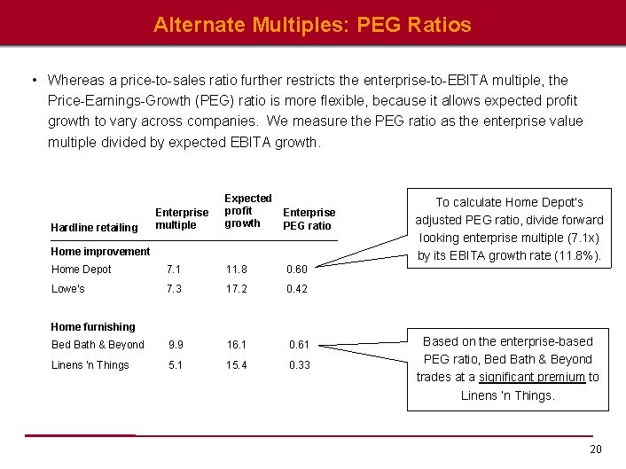
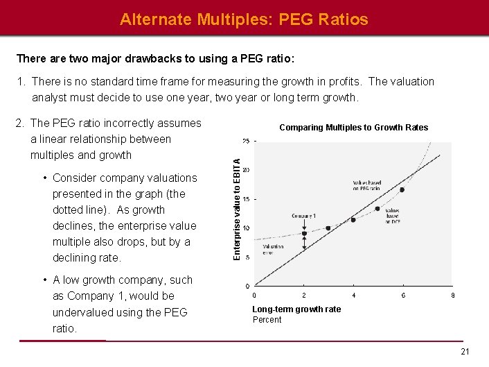
Alternate Multiples: PEG Ratios • Whereas a price-to-sales ratio further restricts the enterprise-to-EBITA multiple, the Price-Earnings-Growth (PEG) ratio is more flexible, because it allows expected profit growth to vary across companies. We measure the PEG ratio as the enterprise value multiple divided by expected EBITA growth. Hardline retailing Enterprise multiple Expected profit growth Enterprise PEG ratio Home improvement Home Depot 7. 1 11. 8 0. 60 Lowe’s 7. 3 17. 2 0. 42 Bed Bath & Beyond 9. 9 16. 1 0. 61 Linens ’n Things 5. 1 15. 4 0. 33 To calculate Home Depot’s adjusted PEG ratio, divide forward looking enterprise multiple (7. 1 x) by its EBITA growth rate (11. 8%). Home furnishing Based on the enterprise-based PEG ratio, Bed Bath & Beyond trades at a significant premium to Linens ‘n Things. 20

Alternate Multiples: PEG Ratios There are two major drawbacks to using a PEG ratio: 1. There is no standard time frame for measuring the growth in profits. The valuation analyst must decide to use one year, two year or long term growth. • Consider company valuations presented in the graph (the dotted line). As growth declines, the enterprise value multiple also drops, but by a declining rate. • A low growth company, such as Company 1, would be undervalued using the PEG ratio. Comparing Multiples to Growth Rates Enterprise value to EBITA 2. The PEG ratio incorrectly assumes a linear relationship between multiples and growth Long-term growth rate Percent 21

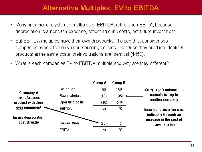
Alternative Multiples: EV to EBITDA • Many financial analysts use multiples of EBITDA, rather than EBITA, because depreciation is a noncash expense, reflecting sunk costs, not future investment. • But EBITDA multiples have their own drawbacks. To see this, consider two companies, who differ only in outsourcing policies. Because they produce identical products at the same costs, their valuations are identical ($150). • What is each companies EV to EBITDA multiple and why are they different? Comp A Company A manufactures product with their own equipment Incurs depreciation cost directly Comp B Revenues 100 Raw materials (10) (35) Operating costs (40) EBITDA 50 25 (30) (5) 20 20 Depreciation EBITA Company B outsources manufacturing to another company Incurs depreciation cost indirectly through an increase in the cost of raw material) 22

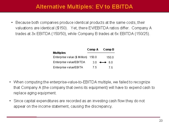
Alternative Multiples: EV to EBITDA • Because both companies produce identical products at the same costs, their valuations are identical ($150). Yet, there EV/EBITDA ratios differ. Company A trades at 3 x EBITDA (150/50), while Company B trades at 6 x EBITDA (150/25). Comp A Multiples Enterprise value ($ Million) 150. 0 Comp B 150. 0 Enterprise value/EBITDA 3. 0 6. 0 Enterprise value/EBITA 7. 5 • When computing the enterprise-value-to-EBITDA multiple, we failed to recognize that Company A (the company that owns its equipment) will have to expend cash to replace aging equipment. • Since capital expenditures are recorded as an investing cash flow they do not appear on the income statement, causing the discrepancy. 23

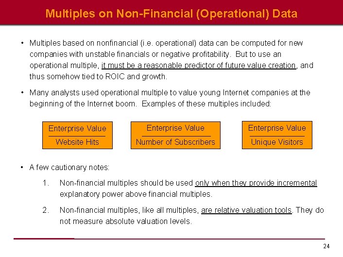
Multiples on Non-Financial (Operational) Data • Multiples based on nonfinancial (i. e. operational) data can be computed for new companies with unstable financials or negative profitability. But to use an operational multiple, it must be a reasonable predictor of future value creation, and thus somehow tied to ROIC and growth. • Many analysts used operational multiple to value young Internet companies at the beginning of the Internet boom. Examples of these multiples included: Enterprise Value Website Hits Number of Subscribers Unique Visitors • A few cautionary notes: 1. Non-financial multiples should be used only when they provide incremental explanatory power above financial multiples. 2. Non-financial multiples, like all multiples, are relative valuation tools. They do not measure absolute valuation levels. 24

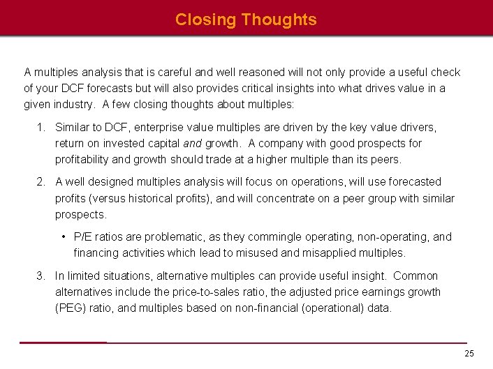
Closing Thoughts A multiples analysis that is careful and well reasoned will not only provide a useful check of your DCF forecasts but will also provides critical insights into what drives value in a given industry. A few closing thoughts about multiples: 1. Similar to DCF, enterprise value multiples are driven by the key value drivers, return on invested capital and growth. A company with good prospects for profitability and growth should trade at a higher multiple than its peers. 2. A well designed multiples analysis will focus on operations, will use forecasted profits (versus historical profits), and will concentrate on a peer group with similar prospects. • P/E ratios are problematic, as they commingle operating, non-operating, and financing activities which lead to misused and misapplied multiples. 3. In limited situations, alternative multiples can provide useful insight. Common alternatives include the price-to-sales ratio, the adjusted price earnings growth (PEG) ratio, and multiples based on non-financial (operational) data. 25